How to Create an Expense Tracker in Excel?

Finance management plays an important role in an organization or in the personal finance of people’s life. In order to manage finances organizations have a finance manager, in the same way individual person can manage their own expenses using an expense manager.

Expense Manager, also known as Expense Tracker is an application or software which is used to keep the records of the inflow and outflow of money. It is used to manage your daily expenses and keep the track of “How much you spend, Over what you have spent”.

For example, In this example we will make an expense tracker using Microsoft Excel, which will automate on the basis of what is entered in the tracker, it will also show how much money is left in each category and will change on the basis of the month selected in the drop-down menu.

Implementation Steps

Step 1: First, we will open the Microsoft Excel application, and we will define the following columns Month, Date, Description, Category, Income, Debits, Balance. You can define your own columns as per your requirements.

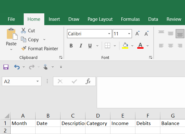
Fig 1 – Expense Tracker Columns

Now, we will turn these columns into tables with all alternating rows. For this, we will select all the columns and go the Format as Table style inside the Home tab of excel and choose any one of the table formatting views you like. Below is the screenshot attached for the same.

Home > Format as Table

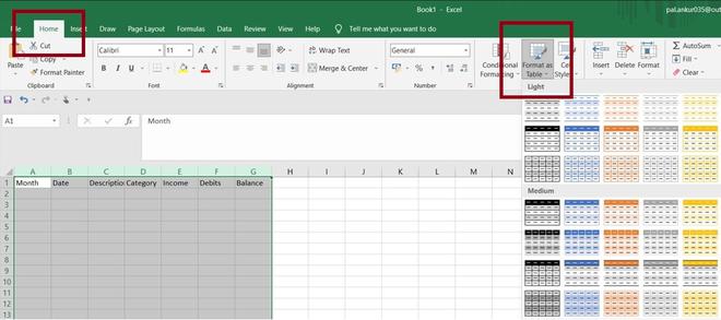
Fig 2 – Format as Table

Once you have selected your table view design a prompt will come there you have to check the checkbox “My table has headers”, which will create the columns of the table as header the header of the table. Click on the OK button.

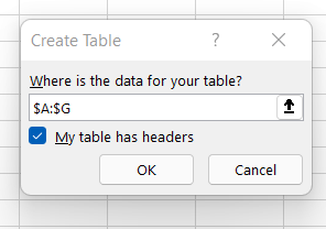
Fig 3 – Table Headers Checkbox

After, you click the OK button tables with headers will be created. And, you will get the table with your columns header.

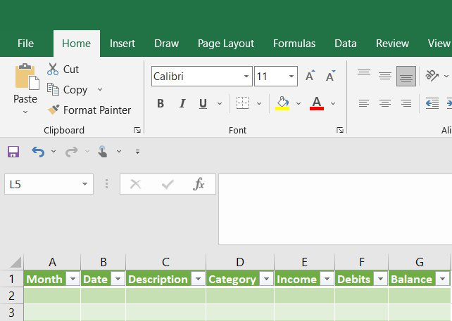
Fig 4 – Expense Table

Step 2: In this step, we will add the necessary formulas and the number formatting to the columns of the table to automate most of the work for us.

First, we will add starting date, and using that we will add up the formulas to our table. For this first, we will add a random date in the date column and hit the enter button.

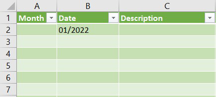
Fig 5 – Date Column

After this, we will change the date format. You can use any format you like, in order to do so, we will select the date column (here, it is column B) and right-click on it and open format cells, there we will go to the date category and choose a date format.

Column B > Right-click > Format Cells > Date > Type

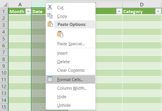
Fig 6 – Date Formatting Option

Now, in the Format Cells tab, we will select the Category as Date and choose a Type of date.

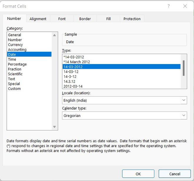
Fig 7 – Date Format Cells

Next, we will set up the formula in the Month column to pull only the month number from the Date column. In order to do this we will write = MONTH([@Date]) inside the month column. The formula will auto-fill the rest of the month rows with the month number from the date column. Whenever we will enter a new date in the date column, it will auto-update the month number according to the date.

=MONTH([@Date])

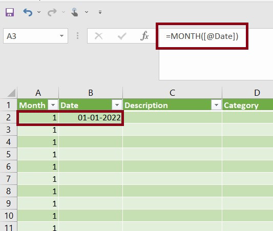
Fig 8 – Auto Month filled according to Date

Step 3: Next, we will add a drop-down menu over the category column so, we can choose a category of expense. For this, we will select the whole category column and then hold the ctrl. key and unselect the column header then from the Data Tab we will select Data validation which is present inside the Data Tools.

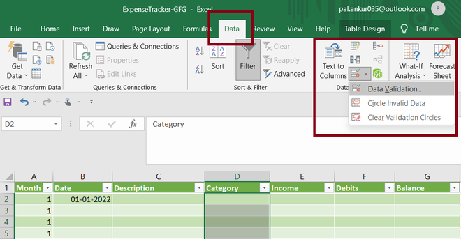
Fig 9 – Category Column

Once you click over the Data Validation option it will open a Data Validation Tab, there inside Validation criteria, in Allow section you have to select List, which is used to create a drop-down list and the list menus should be entered inside the Source section with comma separated the excel will create the list for us.

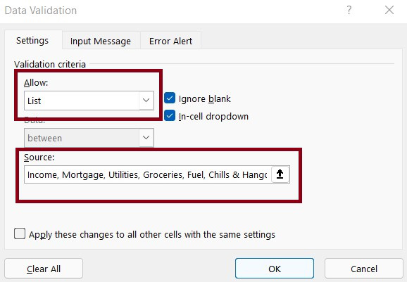
Fig 10 – Data Validation Prompt

You can add the menu list according to your own expenses. Here, we will add Income, Mortgage, Utilities, Groceries, Fuel Chills & hangouts. After adding click on the OK button, Excel will create the drop-down list for all the selected cells and the drop-down menu will be created.

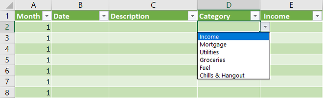
Fig 11 – Categories Menu

After this, we will format the Income, Debits, and Balance columns as currency columns. In order to do so, first, we will select these columns then inside the Home tab we will go to the number section and select the currency, whatever currency you want. In this case, we will choose Indian Rupees currency.

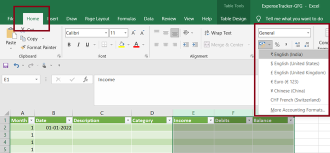
Fig 12 – Income, Debits, and Balance Columns

Step 4: In this step, we will add up the formula to get the running balance. For this, we need to add a starting balance to our expense tracker application. We will add 10000 rupees as Balance and define the Description for this as our starting balance and then we will define the formula to get the running balance.

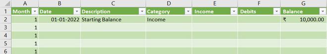
Fig 13 – Starting Balance

Now, we will define the formula in the next cell below balance (cell  G3) to automate the running balance. The formula that will be used is =SUM(G2+[@Income]-[@Debits]).

=SUM(G2+[@Income]-[@Debits])

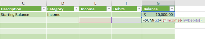
Fig 14 – Formulas For Running Balance

We have to add the formula in the whole column, for this, we will first select the column G3 and press the Ctrl+C key to copy the formula then we will select whole column G and unselect the header and the starting balance cells from column G(here, it is cell G1 & G2) while holding the Ctrl key and then paste the formula using Ctrl+V key, excel will paste it in the whole column.

Once we will paste it, the excel will auto-populate the starting balance of 10000 rupees in the whole of column G same as the month column, But as you update your expenses and income it will calculate the running balance.

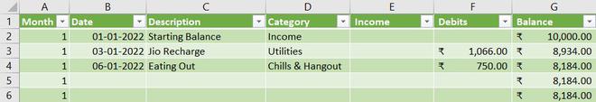
Fig 15 – Auto-Updating Balance

Step 5: In this step, we will create the progress bar which will show how much we have spent in each category and how much income we need in each category. In order to do so, we need to add all the categories in a separate column that we want to track.

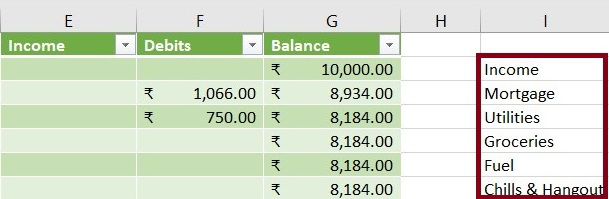
Fig 16 – Tracking Columns

Moving next, we need to add a Total column in cell J1 and add the month number we want to focus on in column I1(here, it’s January so we will add month number a1).

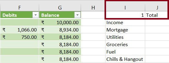
Fig 17 – Total Column & Month Number Column In I1

After this, we need to add the SUMIFS(sum_range, criteria_range1, criteria1, [criteria_range2, criteria2], …) formula for all the columns which we want to keep the track of. We need to write SUMIFS() separately for the Income and Expenses column.

First, we write SUMIFS() for the Income column to keep its track separately with expenses. We will be using the following formula. (Note: Please keep in mind that you will be using the formula according to the columns you have to define)

=SUMIFS(Table1[[#All],[Income]],Table1[[#All],[Month]],I1,Table1[[#All],[Category]],I2)

Fig 18 – SUMIFS() For Income

Now, we will add SUMIFS() formula for our expenses categories. For expenses tracking we will be using the following formula.

=SUMIFS(Table1[[#All],[Debits]],Table1[[#All],[Month]],$I$1,Table1[[#All],[Category]],I3)

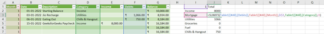
Fig 19 – SUMIFS() For Expenses Categories

After adding this formula we will just drag and drop the formula to all our categories columns we want to track. i.e., Mortgage, Utilities, Groceries, Fuel, and Chills & hangouts. This will update all the expenses according to the months.

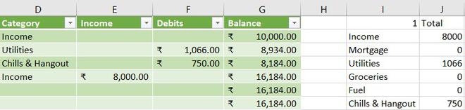
Fig 20 – Expenses Tracking

We can see mortgages, Fuel, and Groceries are coming as 0 since we have not added any expenses in these categories. Now, to enhance it we will change the type of these tracing columns to currencies(Here, In Indian Rupees). In order to do so, we will select all these columns, and then in the Home tab, we will go to the Number section and change the type to currencies.

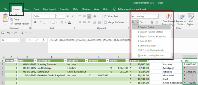
Fig 21 – Change the Type of tracked columns

Step 6: In this step, we will design our progress bar which will show us how much income we will have and how much we got left in each category to spend. Again we will design income separately and the expense categories separately.

Progress bar for Income

We will first select the column having income value. From the Home tab, we will choose Conditional Formatting in the Style section. And, select Data Bars, we will select green bars for the income.

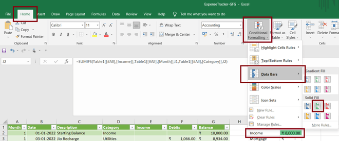
Fig 22 – Progress Bars

We will stretch it a little longer for good visuals. Now, we need to define the rules for it. For this, we will again go to Conditional Formatting and then choose Manage Rules. 

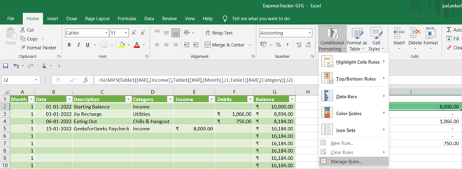
Fig 23 – Manager Rule Tab

We need to update our existing rule which is by default created by excel. We just double-click to open it and update the minimum and maximum value and set its type and number. This will make our progress bar trackable.

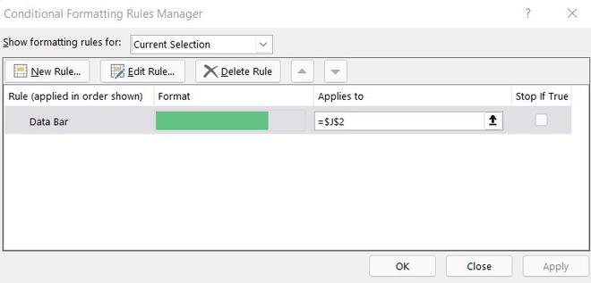
Fig 24 – Default Rules – DATA BAR

We will set the minimum value is 0 and the maximum value as 45000, after we update these values we will press OK and apply our rules.

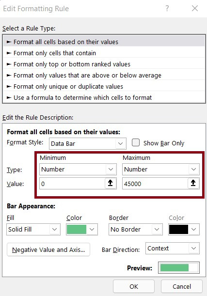
Fig 25 – Manage Rules

After this, we will be done with income and it will look something like this.

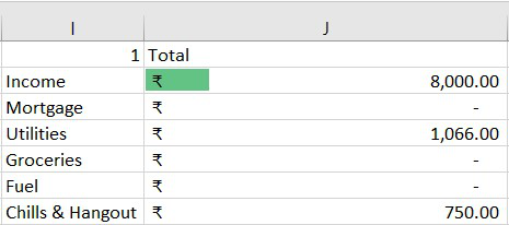
Fig 26 – Income Tracking

The same this we have to do for all of our expenses separately. You can set up the minimum and maximum values according to your requirement. Here, we will be doing expenses tracking in red color with minimum and maximum value as following Mortgage(0, 8000), Utilities(0, 5000), Groceries(0, 5000), Fuel(0, 2000), Chills & Hangout(0, 3000). Once we repeat the same steps for our all-expense we will get something like this.

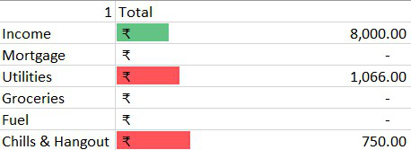
Fig 27 – Expenses Tracking

Step 7: In this step, we will try to enhance our design. We add borders across our tracking table. For this, we will select the whole expense table and drag it down and make a column (Here, it is column H and column K) to equivalent length. You can find it below in the picture.

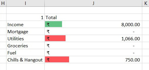
Fig 28 – Tracking Table Border

Moving ahead, we will select the whole table and makes All Borders. For this, we go to the Home tab, and then in the Font section, we will choose the borders option and select All borders it will make borders all around our table.

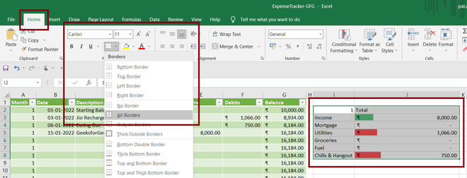
Fig 29 – Tracking Table All Borders

Once we do this we will select the cells around our border which we left in the above step, for that we need to select those cells manually by pressing and holding the ctrl key and selecting the cells.

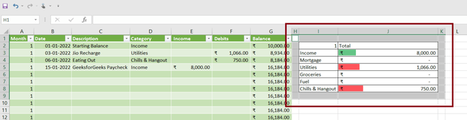
Fig 30 – Cells Selection

Once we select all the cells around our table we fill them with some solid color. For that, we go to the Home tab, and then in the Font section, we will fill the color.

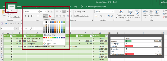
Fig 31 – Filling Cells

Output

Here, we will test our Expense Manager Application. We fill some of the expenses in the month of January and then we will change the month number in Progress Tracking Table and fill for the month of February.