How to Create a Stem-and-Leaf Plot in Excel?

Stem and Leaf plot is a histogram tabulation of data. Stem and leaf plot is better for data visualization and cleanliness of the data in a certified range. The plot helps determine the frequency distribution of the data. In this article, we will learn how to create a stem and leaf plot in excel. 

Stem and Leaf Analogy

The stem is the main upholding of a tree. The stem divides into branches and branches contain leaves. The concept in the Stem and Leaf plot in excel is also quite similar to it. For example, you are given the data of numbers, 12, 12, 13,  53. These numbers can be better represented as 1 -> 2 2 3 and 5-> 3 where 1 5 contributes to the stem and 2 2 3 3 contributes to the leaves. 

For example, data set is 12, 220, 15, 221, 20, 20, 23. 

The Stem and Leaf plot for the above data set will be: 

                                                 1    |      2  5  

                                                 2    |      0  0  3

                                                 22  |      0  1

Some important function

Before creating a stem and leaf plot in excel. We will quickly summarise the formulas required to make a stem and leaf plot. 

1. =FLOOR.MATH(): The floor function returns an integer i.e. the greatest integer of x. Three arguments can be passed in the floor function, but the minimum requirement is the first argument. 

Syntax: 

=FLOOR.MATH(number, [significance], [mode]). 

For stem and leaf plots, only the first argument will be used in our use case. For example, =FLOOR.MATH(23.9) is equal to 23. 

2. =RIGHT(): The right function returns a substring from the right. Two arguments can be passed in the right function, but the minimum requirement is the first argument. 

Syntax: 

=RIGHT(number, [number_of_characters_from_the_right]).

For example, =RIGHT(“geeks”, 2), is equal to “ks”. 

3. =REPT(): The rept function returns a string repeated a given number of times. Two arguments can be passed in the rept function, and both arguments are mandatory. 

Syntax: 

=REPT(text, number_of_times_text_to_be_repeated). 

For example, =REPT(0, 4), is equal to 0000. 

4. =COUNT(): The count function counts the number of cells that meet a given condition. Two arguments can be passed in the count function, and both arguments are mandatory. 

Syntax: 

=COUNTIF(range_of_selected_cells, condition_specified). 

For example, A2 = 2, A3 = 2, A4 = 12, A4 = 5. =COUNTIF(A2:A4, 2) is equal to 2. 

Creating a Stem and Leaf Plot 

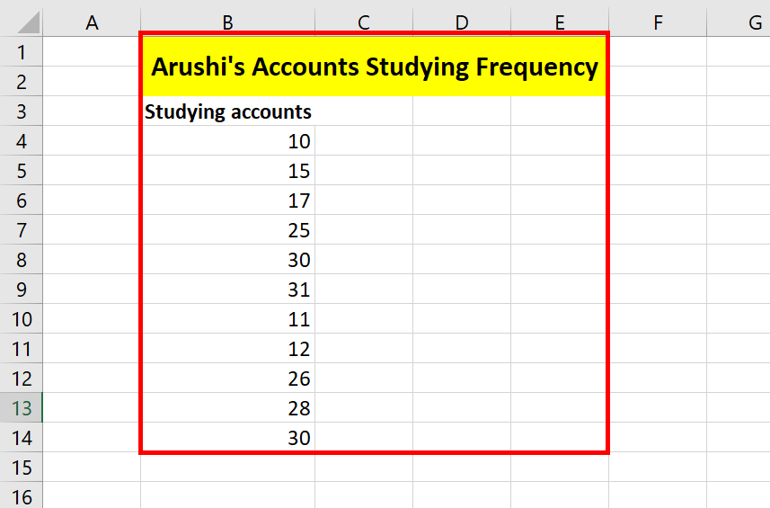
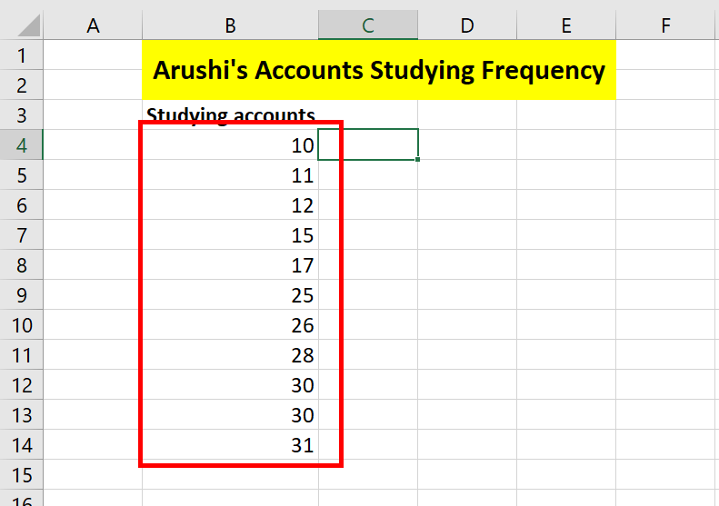
Now we will create a stem and leaf plot in excel. Consider a data set, Arushi is an aspiring Chartered Accountant. She studies accounts on random days in a month. Arushi has prepared data of two months, in which she mentions the days she use to study accounts. Help Arushi make a Stem and Leaf plot so that she can present the quantitative data in an organized manner. 

Following are the steps: 

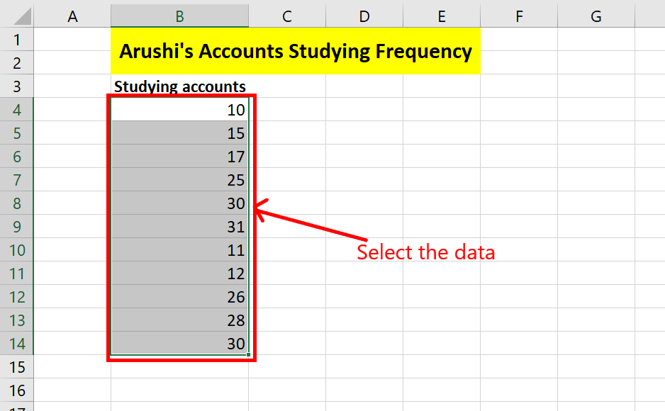
Step 1: Firstly, you need to sort the data. Select the data, B4:B14. 

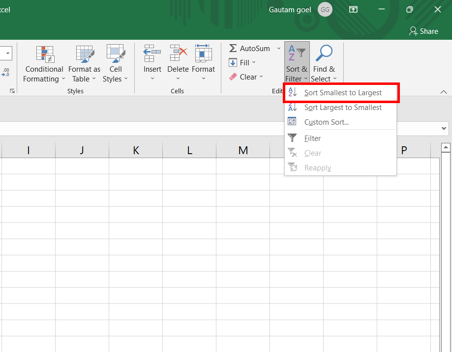
Step 2: Go to Home tab, under editing section, in Sort and Filter, select Sort Smallest to Largest.

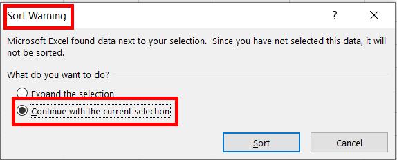
Step 3: Sort Warning dialogue box appears. Select Continue with the Current Selection. Click on the Sort button. 

Step 4: The selected data got sorted. 

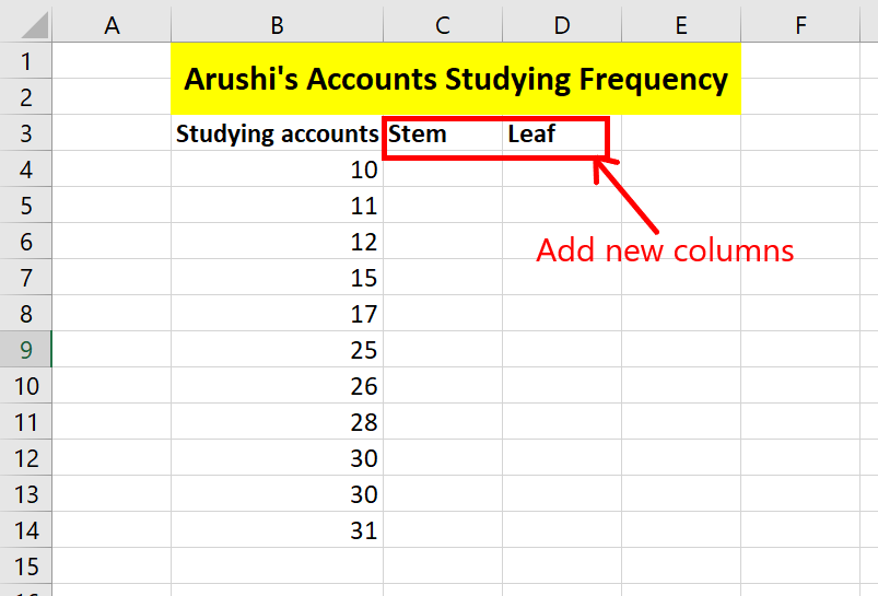
Step 5: Add two new columns name Stem and Leaf. 

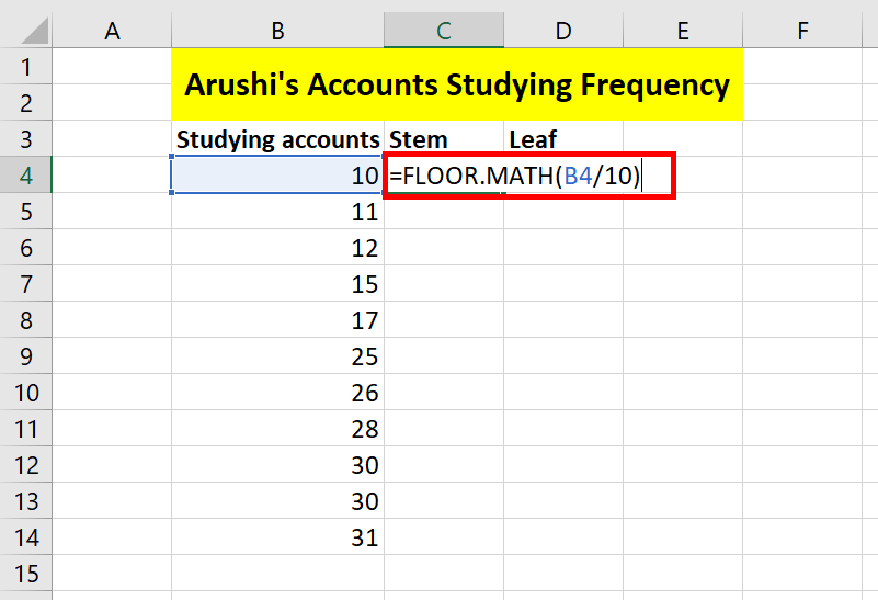
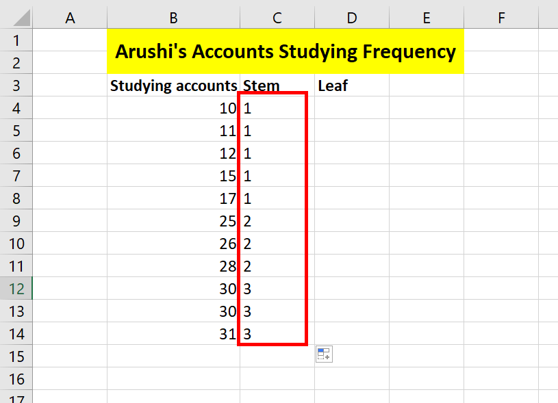
Step 6: In cell C4, write the formula =FLOOR.MATH(B4/10). The formula divides the selected cell by 10 and changes it to its floor value. 

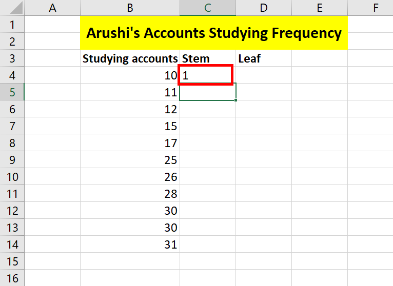
Step 7: Press Enter. The required output is attained. For example, =FLOOR.MATH(10/10) is equal to 1. 

Step 8: Current active cell is C4. Drag and drop from C4 to C14. The same formula gets copied in C5:C14.

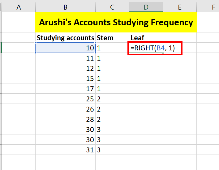
Step 9: In cell D4, write the formula =RIGHT(B4, 1). The formula gives the last character of cell B4. 

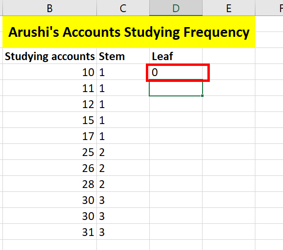
Step 10: Press Enter. The required output is attained. For example, =RIGHT(10, 1) is equal to 0. 

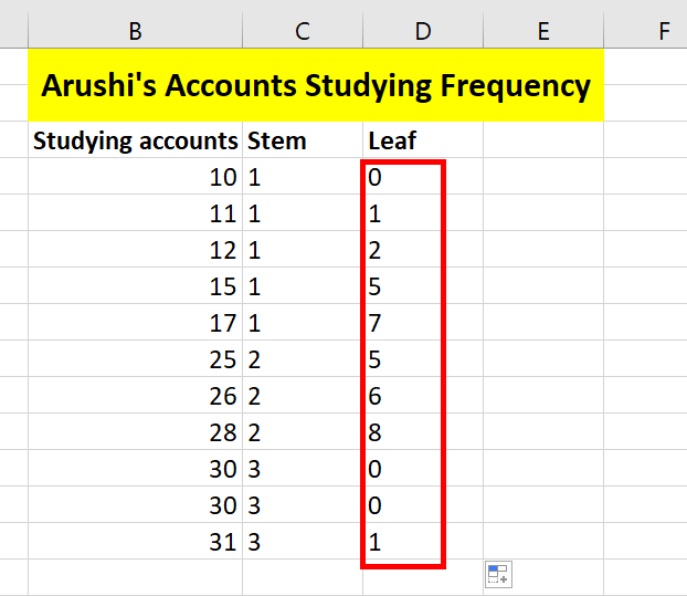
Step 11: Current active cell is D4. Drag and drop from D4 to D14. The same formula gets copied in D5:D14.

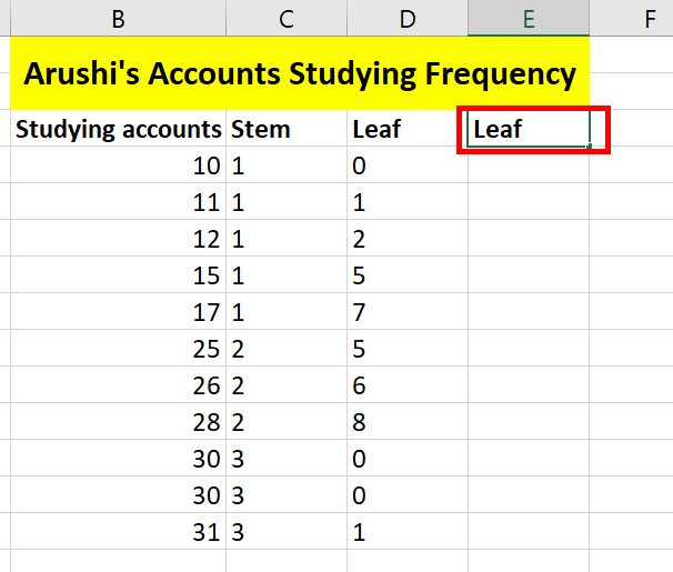
Step 12: Add a new column in cell E3, name Leaf. 

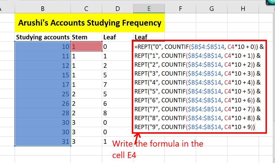
Step 13: In cell E4, write the formula =REPT(“0”, COUNTIF($B$4:$B$14, C4*10 + 0)) & REPT(“1”, COUNTIF($B$4:$B$14, C4*10 + 1)) & REPT(“2”, COUNTIF($B$4:$B$14, C4*10 + 2)) & REPT(“3”, COUNTIF($B$4:$B$14, C4*10 + 3)) & REPT(“4”, COUNTIF($B$4:$B$14, C4*10 + 4)) & REPT(“5”, COUNTIF($B$4:$B$14, C4*10 + 5)) & REPT(“6”, COUNTIF($B$4:$B$14, C4*10 + 6)) & REPT(“7”, COUNTIF($B$4:$B$14, C4*10 + 7)) & REPT(“8”, COUNTIF($B$4:$B$14, C4*10 + 8)) & REPT(“9”, COUNTIF($B$4:$B$14, C4*10 + 9)). This formula might seem complicated but its very easy. Understand, the sub formula of it i.e.  =REPT(“0”, COUNTIF($B$4:$B$14, C4*10 + 0)). This sub formula simply counts the number of 10 in the data set and then =REPT() function repeats the number of 0’s in it. Now, its easy, repeat the same subformula for all and then you will concatenate all possible number of repetitions of number i.e. 10, 11, 12, 13….19.

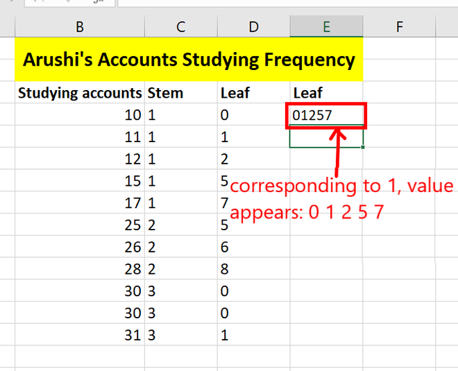
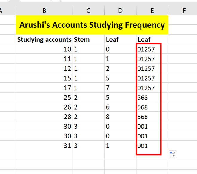
Step 14: Press Enter. Copy the same formula to the range E4:E14.

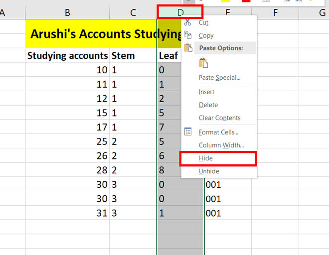
Step 15: Your stem and leaf plot is ready. You can still do some customizations. You can hide column D from your worksheet i.e. the first leaf name column. Right-click on Column D and click on the hide button. 

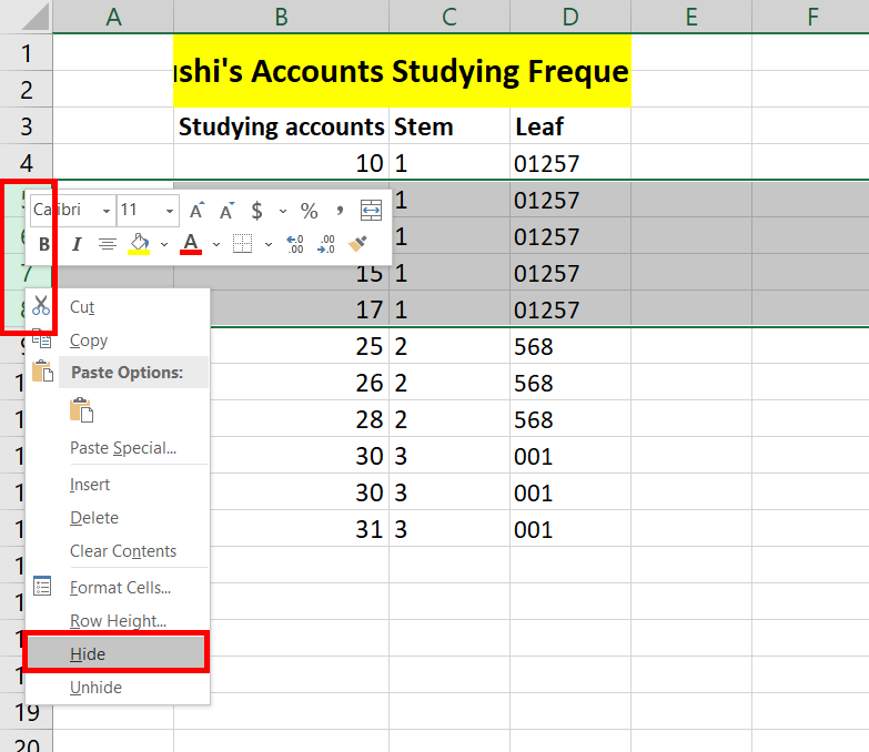
Step 16: Similarly, you can hide the same values in the stem column. Select the required rows and right-click on them. Click on the hide button. 

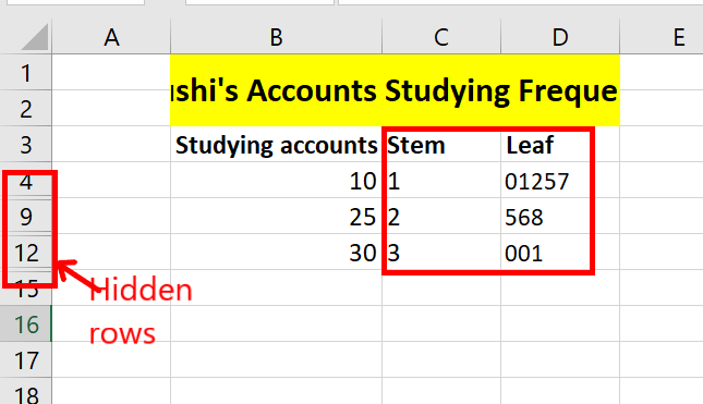
Step 17: Your Stem and Leaf plot is ready.