How to Create a Drop-Down List in Excel

A drop-down list offers users a selection from predefined options, commonly used on sites/applications for easy navigation. Dynamic arrays in Excel 365 allow us to create drop-down lists quickly, without complex setups.

How to Create Drop-Down List in Excel

In this segment, you will learn how to make an Excel drop-down list in quick and easy steps.

5 Ways to Create a Drop-Down List in Excel

Create Drop-Down List in Excel Using Data from Cells

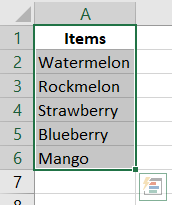
Suppose you have a column of cells as displayed below:

Drop Down List in Excel

Here are the steps toward making an Excel Drop Down List:

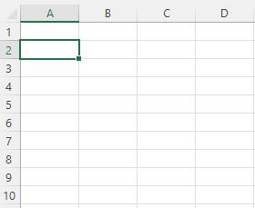
Step 1: Select the Cell

Select Cell where you need to make the drop-down list.

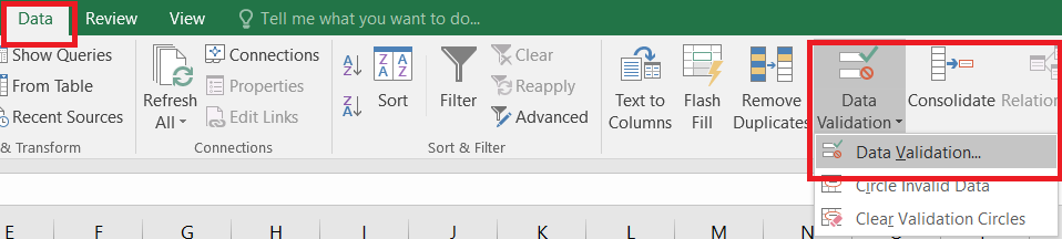
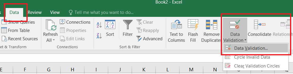
Step 2: Go to the Data Tab and Select Data Validation in Data Tools Group

Go to Data –> Data Tools –> Data Validation.

Excel Tool Bar

Step 3: Select List as the Validation Model

In the Data Validation popup, inside the Settings tab, select List as the Validation Criteria.

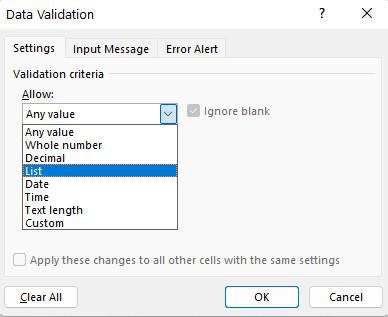
• When you select List, the Source field shows up.
• In the source field, enter =$A$2:$A$6, or essentially click in the Source field and select the cells utilizing the mouse and snap OK.

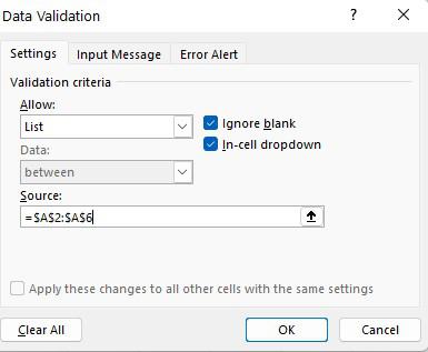
• This will then embed a drop-down list.

Step 4: Preview the Drop-Down List in Excel

Ensure that the In-cell dropdown choice is checked (which is checked, by default). On the off chance that this choice is uncontrolled, the cell doesn’t show a drop-down. In any case, you can physically enter the qualities in the rundown.

Final Drop Down List

Create Drop-Down in Excel By Entering Data Manually

In the above model, cell references are utilized in the Source field. You can likewise add things straight by entering them physically in the source field. This is the way you can straightforwardly enter it in the information approval source field:

Step 1: Select the Cell

Select a cell where you need to make the drop-down list (cell A2 in this model).

Step 2: Go to the Data Tab and Select Data Validation in the Data Tools Group

Go to Data –> Data Tools –> Data Validation.

Excel Tool Bar

Step 3: Select List in Validation Criteria

In the Data Validation popup, inside the Settings tab, select List as the Validation Criteria. When you select List, the source field shows up.

• In the Source field, enter Yes, and No.

• Make sure that the In-cell dropdown option is checked. Click OK.

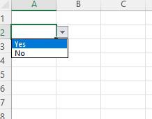
This will make a drop-down list in the chosen cell. Every one of the things recorded in the source field, isolated by a comma, is recorded in various lines in the drop-down menu.

Note: If you need to make drop-down records in different cells at one go, select every one of the cells where you need to make it and afterward follow the above advances.

Create drop-down List in Excel Using Formulas

Aside from choosing from cells and entering information physically, you can likewise involve a recipe in the source field to make an Excel drop-down list. Any recipe that profits a rundown of values can be utilized to make a drop-down list in Excel.

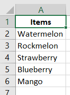
For instance, assume you have the informational index as displayed underneath:

Here are the moves toward making an Excel drop-down list utilizing the OFFSET formula:

Step 1: Select a Cell

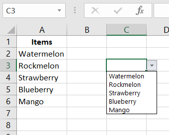
Select a cell where you need to make the drop-down list (cell C3 in this model).

Step 2: Go to the Data Tab and Select Data Validation in the Data Tools Selection

Go to Data –> Data Tools –> Data Validation.

Excel Tool Bar

Step 3: Select List in Validation Criteria

In the Data Validation popup, inside the Settings tab, select List as the Validation Criteria. When you select List, the source field shows up.

• In the Source field, enter the accompanying equation: “=OFFSET($A$2,0,0,5)”. Ensure that the In-cell dropdown choice is checked.

• Click OK. This will make a drop-down list that runs down all the organic product names (as displayed underneath).

Final Drop Down List

Note: If you need to make a drop-down list in different cells at one go, select every one of the cells where you need to make it and afterward follow the above advances. Ensure that the cell references are outright (like $A$2) and not a family member (like A2, or A$2, or $A2).

How does the OFFSET formula Work?

In the above case, we utilized an OFFSET capability to make the drop-down list. It returns a rundown of things from the reach A2:A6. Here is the sentence structure of the OFFSET capability: =OFFSET(reference, lines, cols, [height], [width])

It takes five contentions, where we determined the reference as A2 (the beginning stage of the rundown). Lines/Cols are determined as 0 as we would rather not offset the reference cell. The level is determined, however, 5, as there may be five components in the rundown.

Create a Dynamic Drop-down List that Automatically Expands in Excel

The above method of utilizing an equation to make a drop-down rundown can be stretched out to make a powerful drop-down list too. On the off chance that you utilize the OFFSET capability, as displayed above, regardless of whether you add more things to the rundown, the drop-down won’t refresh consequently. You should physically refresh it each time you change the rundown. Here is a method for making it dynamic .

Step 1: Select the Cell

Select a cell where you want to create the drop-down list (cell C2 in this example).

Step 2: Go to the Data Tab and Select Data Validation in the Data Tools Selection

Go to Data –> Data Tools –> Data Validation.

Excel ToolBar

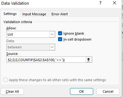
Step 3: Select List in Validation Criteria and Enter the formula

In the Data Validation popup, within the Settings tab, select List as the Validation criteria. As soon as you select List, the source field appears. In the source field, enter the accompanying recipe:

=OFFSET($A$2,0,0,COUNTIF($A$2:$A$100,”<>”))

Step 4: Click OK

Ensure that the In-cell drop-down choice is checked. Click OK.

In this equation, we have supplanted contention 5 with COUNTIF($A$2:$A$100,”<>”). The COUNTIF capability includes the non-clear cells in the reach A2:A100. Consequently, the OFFSET capability changes itself to incorporate every one of the non-clear cells.

Select Multiple Items from a Drop Down List in Excel

Now and again, it’s difficult to tell which cells contain the drop-down list. Thus, it’s a good idea to stamp these cells by either giving them an unmistakable boundary or a foundation tone. Rather than physically checking every one of the phones, there is a fast method for choosing every one of the phones that has drop-down records (or any information approval rule) in it.

Step 1: Go to the Home Tab, Select Find and Select, and Choose Go to Special

• Go to Home  –> Find & Select –> Go To Special.

Step 2: Select Data Validation and Click OK

• In the Go To Special exchange box, select Data Validation. Click OK.

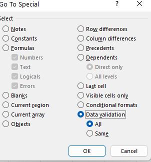
• Information approval has two choices: All and the Same. All would choose every one of the cells that have an information approval rule applied to it. The same would choose just those cells that have similar information approval as that of the dynamic cell.

How to Create a Drop-Down List in Excel with Multiple Selections

Step 1: Select the Cell Range

Choose the cells where you want the drop-down list to appear.

Select the Cell

Step 2: Go to the Data Tab

Navigate to the “Data” tab on the Excel ribbon.

Step 3: Select the Data Validation Option

Click on the Data Validation option in the Data Tools group.

Excel Toolbar

Step 4: In the Data Validation Dialog Box, Go to Settings

In the Data Validation dialog box, go to the Settings tab.

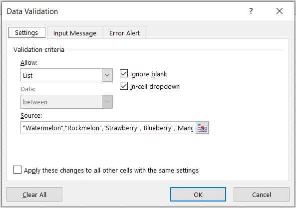
Step 5: Select List in the Allow drop-down

In the Allow dropdown, select List.

Step 6: Enter the Values in the Source Field

In the Source field, enter the values you want in your list, separated by commas. For example, if you want to have a list with the options “Option 1”, “Option 2”, and “Option 3”, you would enter: Option 1, Option 2, Option 3.

Data Validation

Step 7: Enable Multi-Selection and Click ok

To allow multiple selections, check the box that says “In-cell dropdown.”

Step 8: Preview Result

Final Drop Down List

Conclusion

Creating drop-down lists in Excel is like giving your spreadsheet superpowers. It lets people choose from a set of options you’ve already decided, making data entry and dashboard building easier.

The article talks about different ways to make these drop-down lists, using things like data from cells, typing options manually, or even using a smart formula (OFFSET) for a list that automatically grows. There’s also a cool trick to select multiple items from the list.

How to Create a Drop Down List in Excel – FAQs

How do I create a drop-down list in Excel?

Steps to create a drop-down list in Excel are:

1. Select the Cell(s): Click on the cell or cells where you want the drop-down list.
2. Go to the “Data” Tab: Navigate to the “Data” tab on the Excel ribbon.
3. Choose “Data Validation”: Click on “Data Validation” in the “Data Tools” group.
4. Set up Validation Criteria: In the “Data Validation” dialog box, go to the “Settings” tab.
5. Choose “List” in the “Allow” dropdown.
6. Specify the Source: In the “Source” field, enter the values you want in your list, separated by commas.
7. Click OK.

How do I create a drop-down list in Excel with multiple selections?

Steps to create a drop-down list in Excel with multiple selections are:

1. Select Cells: Click on the cells where you want the list.
2. Go to “Data” Tab: Visit the “Data” tab in Excel.
3. Choose “Data Validation”: Click on “Data Validation.”
4. Set up List: Enter or select your options, separated by commas.
5. Enable Multi-Selection: Check “In-cell dropdown.”
6. Apply: Click “OK.”

How do I create a drop-down list and autofill in Excel?

Steps to create a drop-down list and autofill in Excel are:

1. Select the Cell(s): Click on the cell or cells where you want the drop-down list.
2. Go to the “Data” Tab: Navigate to the “Data” tab on the Excel ribbon.
3. Choose “Data Validation”: Click on “Data Validation” in the “Data Tools” group.
4. Set up Validation Criteria: In the “Data Validation” dialog box, go to the “Settings” tab.
5. Choose “List” in the “Allow” dropdown.
6. Specify the source of your list (values separated by commas or a range).
7. Enable Autofill: Check the “In-cell dropdown” option.
8. Optionally, check “Show error alert” to guide users if needed.
9. Click OK: Click “OK” to apply the data validation and create the drop-down list.

How to edit a drop-down list in Excel?

To edit a drop-down list in Excel:

Go to Data > Data Tools Selection > Data Validation. And in the Settings tab, click the Source box, and in the Source box change the items as per your need.

How can I customize a drop-down list in Excel?

To customize a drop-down list in Excel:

1. Select the cell for the list.
2. Go to Data > Data Validation.
3. Choose “List” in Allow box.
4. Enter range for options or type them separated by commas.
5. Click OK.