How to Compare Two Columns in Excel : Easy and Quick Methods

Excel provides various functions and methods by which we can compare two columns and identify matching and mismatching data. Working with a very large Excel dataset, comparing two different columns, and recording the result as Matched or Not Matched can be very time-consuming. It is simple to compare columns in small tables but it becomes complicated when you need to compare two columns in a large spreadsheet. Comparing the columns manually is a time-consuming approach that can be avoided with the application of some fundamental knowledge of Excel.

Why Compare Two Columns in Excel

Excel is a versatile tool that stores data and manipulates data for better decision-making. We are required to compare Excel columns data for the following reasons:

• To find the unique value in the dataset.
• To remove the identical data values from the dataset.
• To reduce the size of the dataset.
• To speed up the processing time for other Excel operations by reducing its size and removing identical data values.

How to Compare Two Columns in Excel

There are many different ways to compare your data when it is present in two different columns, tables, or spreadsheets to make sure that there shouldn’t be any missing or duplicate data present in the columns.

Below are some methods to compare two columns :

• Highlighting the unique or duplicate values in each column using Functions
• Display Unique or duplicate using conditional formatting or formulas.
• Comparison through row by row
• Using LOOKUP formulas.

In this example, we will be using random cities’ names in two different columns and comparing them to find duplicate or unique cities’ names. For this example, we will create the following dataset. The dataset will contain two columns as Cities A and Cities B, which will contain random names of cities. Below is the screenshot of the dataset attached.

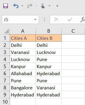
Fig 1 – Dataset

Compare Two Columns in Excel using Conditional Formatting

In this method, we will the Conditional Formatting rules provided by Excel to compare the two columns and highlight the DUPLICATE DATA between the two columns.

Step 1: Select the data

First, we will select the data cells of Excel for which we want to compare the data.

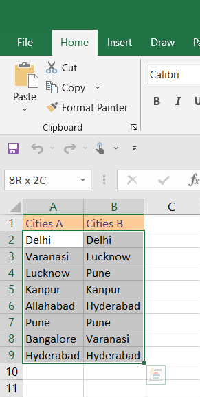
Fig 2 – Select the data cells

Step 2: Conditional Formatting

In this step, we will do the conditional formatting for our selected cell’s data and set the rules for highlighting the duplicate values. For this go to Home > Styles > Conditional Formatting > Highlight Cells Rules > Duplicate Values.

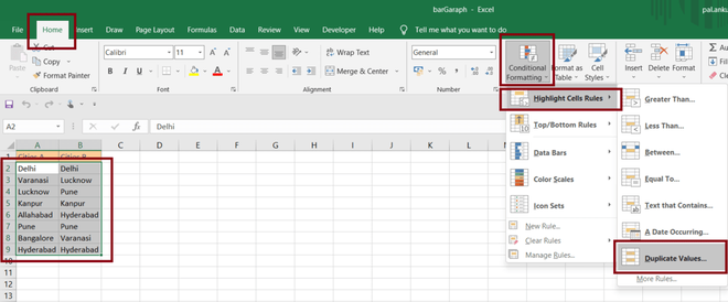
Fig 3 – Conditional Formatting

Once we click on Duplicate Values, excel will pop up a tab asking for a formatting rule. We can select the according to our requirements.

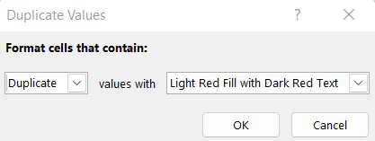
Fig 4 – Formatting Rule

After setting the rule(Here, Light Red color for cells having duplicate data values) we need to click on the OK button.

Step 3: Output

Once we set the formatting rules and click on the OK button, excel will automatically Highlight the cells according to the formatting rule.

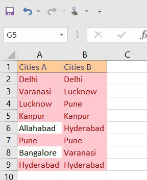
Fig 5 – Output

Highlight Unique Data

In this method, we will use the Conditional Formatting rules provided by Excel to compare the two columns and highlight the UNIQUE DATA between the two columns.

We are required to repeat the same steps as we did in Method 1. But we need to make sure, to change the formatting rule. This time we need to format the cells that contain unique elements, not duplicate elements.

Note: Keep in mind to change the formatting rule for unique data.

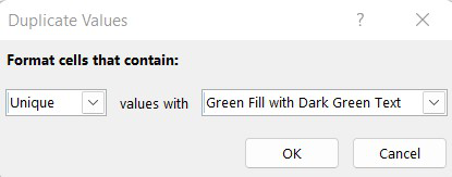
Fig 6 – Formatting rule for a unique element

Output

Once we will change the rule for unique element comparison and click on the OK button, Excel will automatically update the sheet according to the unique element.

Compare Two Columns in Excel Using Equals Operator

In this method, we will create one more column in our existing dataset as Result which will be used for storing the matched and unmatched responses.

Step 1: Add an Excel New Column

In this step, we will add a new column as “Result” for adding the response as TRUE or FALSE.

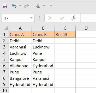
Fig 8 – Add Result Column

Step 2: Adding Comparison Formula

In this step, we will add a formula in our Result column to compare whether the two columns contain equal data or not.

=A2=B2(We are using A2 and B2 cells for comparison, you need to change according to your own cells).

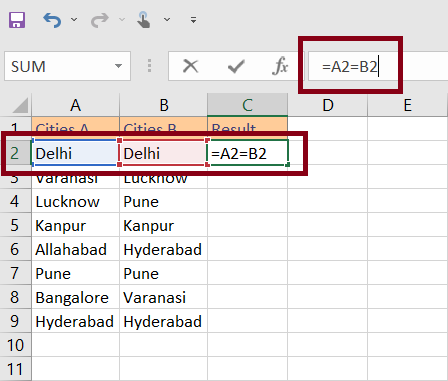
Fig 9 – Adding rules for true or false

After using formula in one row, we need to fill the same formula for all the rows. To use the same formula in all rows, Select the bottom right corner of the cell(Here, C2) and pull it down to the cell. Excel will fill the same formula in all the rows.

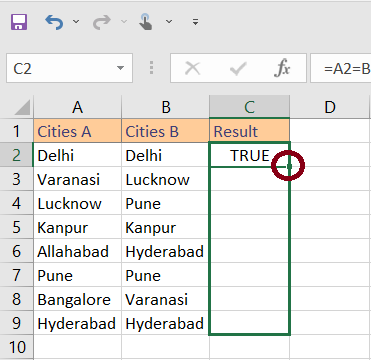
Fig 10 – Fill formula in all rows

Step 3: Output

Once we have our comparison formula filled in all the rows, excel will automatically fill TRUE for matched and FALSE for unmatched entities.

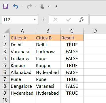
Fig 11 – Output

Compare Two Columns in Excel Using the IF Condition

You can also use the IF condition to compare two columns in Excel. The Formula that can be used is =IF(A2=B2,”MATCH”,” “). It will return the result as MATCH against the rows that contain, matching values, and the remaining rows will show Not Match.

Compare Two Columns in Excel Using the EXACT() Function

The EXACT() Function is used to compare two text strings and returns TRUE if they are the same and FALSE if they are not the same. EXACT is case-sensitive but it ignores formatting differences.

Syntax: =EXACT(text1,text2)

It takes two arguments text1, and text2.

Let’s consider the below Example. There are two columns Cities1 and Cities2. The formula =IF(EXACT(A2,B2),”Match”,”Not match”)

The EXACT() returns values as True or False. The execution of the formula would be: First, the inner function would be executed, and the result returned.

Using the Lookup Function to Compare Two Columns

The LOOKUP function is used to search for a particular value in a particular row or column and return the result from another row or column. Excel has various lookups such as VLOOKUP (V stands for vertical), HLOOKUP (H stands for horizontal), and XLOOKUP (combination of both VLOOKUP and HLOOKUP).

Let’s see the below example to compare two columns using VLOOKUP.

Where Column A consists of a list of exams given by a student and Column B is a list of

subjects that students passed. The result sheet should contain a list of all the subjects. The VLOOKUP() is applied in cell C2 as =VLOOKUP(A2, $B$2:$B$4,1,0).

Drag the formula to apply it in the cell below C2. You will find the result in column C with the subjects that are cleared and those that have not been passed as N/A.

FAQs on Comparing Two Columns in Excel

How to compare two Columns in Excel easily?

Follow the below steps to compare two columns:

Step 1: Select both columns of data.

Step 2: Go to Home.

Step 3: Then click on Find & Select.

Step 4: Now Go To Special > Select row Differences.

Step 5: Click OK.

How to compare two cells in Excel?

Comparing two cells can be easily understood by comparing two columns in Excel row by row except that you don’t have to copy the formulas down to other cells in the column.

For Example: When you want to compare cells A1 and B1, use below-mentioned formulas.

For matches: =IF(A1=B1,”Match”,” “)

For Difference : =IF(A1<>B1, “Difference”,” “)

How to compare multiple columns for matches in the same row?

Find rows with the same values in all columns.

If your table has three or more columns and you want to find the ones that have the same values in all cells, an IF formula with an AND statement.

=IF(AND(A2=B2, A2=C2), Full match”, “”)

And if your table has a lot of columns, the better solution is to use the COUNTIF function.

=IF(COUNTIF($A2:$E2, $A2)=5,” Full match”, “”), where 5 is the number of columns you are comparing.

Can we compare two columns in Excel using the Index-Match function?

Sometimes, You need to match two columns in two different tables and pull matching entries from the comparing table. Use the INDEX-MATCH formula for comparing the values and to pull the values from the other table.

Formula : =INDEX( $B$2:$B$4,MATCH($D2,$A$2:$A$4,0))