How to Compare Two Columns and Delete Duplicates in Excel?

Many a time while working with Microsoft Excel or MS Excel or Excel, we came up with a situation where we have duplicate values in columns and rows and the first task is to remove all the duplicates before proceeding to the next step. But before removing duplicates, we need to find out where these duplicates are present and for that we need to compare columns and rows to find the duplicate entry. After the duplicate values are found, we need to highlight them and remove them. The above process will be explained using excel commands.

Comparing two columns in MS Excel

Follow the following steps to compare two columns in excel:

Note: This tutorial is for MS Excel 2013. Steps can be different or the same for other versions of Excel.

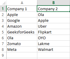
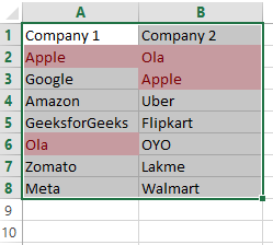
Step 1: Open the Excel file on which you want to compare the columns. For Example, your data can look like this

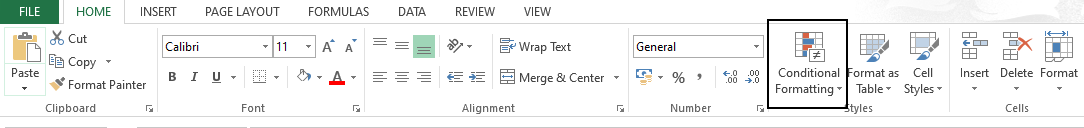
Step 2: Select the columns and go to the Home tab > Style group> Conditional Formatting i.e first click on Home tab, then go to Style group and then select Conditional Formatting (as shown in the image below). Conditional formatting allows users to automatically apply formattings such as changing colors, data bars, and icons in the cells based on cell value.

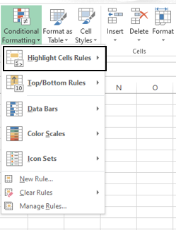
Step 3:  After clicking on Conditional Formatting, a drop-down menu will appear. From the menu ribbon select the Highlight Cells Rules

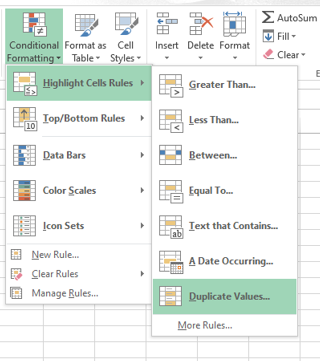
Step 4: After selecting Highlight Cell Rule another drop down will appear and, select Duplicate Values

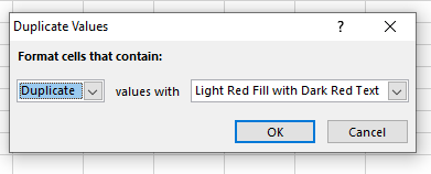
Step 5: After selecting Duplicate Values, a dialogue box (given below) will appear. In the first space fill Duplicate and in the other space fill the color options that you want to duplicate values to be highlighted in. And click OK. The purpose of this step is to highlight the duplicate values. 

Step 6: After clicking OK. The duplicated values are highlighted. 

Removing Duplicate Values

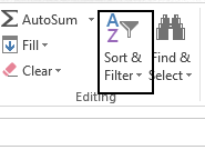
Step 1: We’ll be adding a filter to columns A and B and for that go to Home Tab> Editing Group> Sort & Filter. Here, Sort & Filter will help to apply various filters such as sort in ascending, descending order and sort by color, and much more.

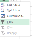
Step 2: After clicking on Sort & Filter, a dialogue box will appear (as shown below). From the dialogue box, select Filter

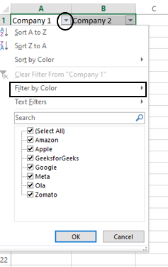
Step 3: You’ll see a downward arrow in the first cell of all the selected columns. After clicking on the downward arrow, a dialogue box will appear(as shown below). Select Filter by Color option.  

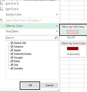
Step 4: In the Filter by Color, select Filter by Cell Color. Remember, here the default color is taken, if you want to take a different color then choose that cell color. And then press OK.

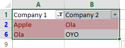
The result will look like this. The duplicate values are highlighted in Column A because the filter is applied to Column A and if you want to highlight the duplicate values from column B, then apply the filter in Column B.

Step 5: Select the cells from Column A that are colored and right-click, a dialogue box will appear(as shown below) and from the dialogue box select Clear Contents

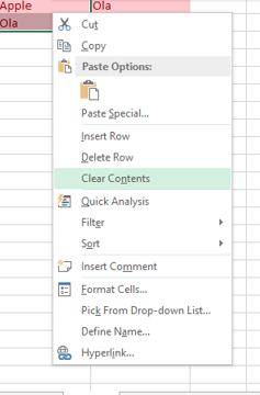
All the duplicate contents will be deleted.