How to change angle of 3D plot in Python?

Prerequisites: Matplotlib, NumPy

In this article, we will see how can we can view our graph from different angles, Here we use three different methods to plot our graph. Before starting let’s see some basic concepts of the required module for this objective.

• Matplotlib is a multi-platform data visualization library built on NumPy arrays and designed to work with the broader SciPy stack
• Numpy is a general-purpose array-processing package. It provides a high-performance multidimensional array object, and tools for working with these arrays. It is the fundamental package for scientific computing with Python
• mpl_toolkits provides some basic 3D plotting (scatter, surf, line, mesh) tools.

Approach:

• Import required library.
• Create a figure.
• Create a datasheet.
• Change angle of the 3D plot
• Show Graph.

Step 1: Import libraries.

Python3

from mpl_toolkits import mplot3d
import numpy as np
import matplotlib.pyplot as plt

Step 2: Plotting 3-D axis figure.

Python3

from mpl_toolkits import mplot3d
import numpy as np
import matplotlib.pyplot as plt

fig = plt.figure(figsize = (8, 8))
ax = plt.axes(projection = '3d')

Step 3: Creating a Datasheet for all the 3-axis of the sample.

Python3

from mpl_toolkits import mplot3d
import numpy as np
import matplotlib.pyplot as plt

fig = plt.figure(figsize = (8, 8))
ax = plt.axes(projection = '3d')

# Data for a three-dimensional line
z = np.linspace(0, 15, 1000)
x = np.sin(z)
y = np.cos(z)
ax.plot3D(x, y, z, 'green')

Step 4: Use view_init() can be used to rotate the axes programmatically.

Syntax: view_init(elev, azim)

Parameters: 

• ‘elev’ stores the elevation angle in the z plane.
• ‘azim’ stores the azimuth angle in the x,y plane.D constructor.

Python3

from mpl_toolkits import mplot3d
import numpy as np
import matplotlib.pyplot as plt

fig = plt.figure(figsize = (8,8))
ax = plt.axes(projection = '3d')

# Data for a three-dimensional line
z = np.linspace(0, 15, 1000)
x = np.sin(z)
y = np.cos(z)
ax.plot3D(x, y, z, 'green')

ax.view_init(-140, 60)

Below is the full Implementation:

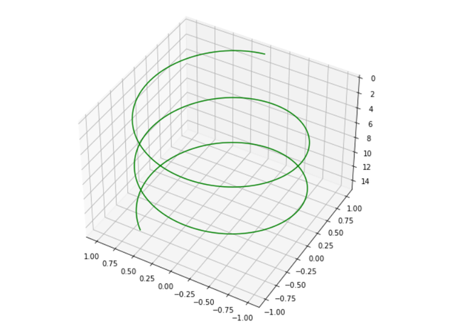
Example 1: In this example, we will plot a curve graph with an elevated angle of -140 degrees and a horizontal angle of 60 degrees.

Python3

from mpl_toolkits import mplot3d
import numpy as np
import matplotlib.pyplot as plt

fig = plt.figure(figsize = (8,8))
ax = plt.axes(projection = '3d')

# Data for a three-dimensional line
z = np.linspace(0, 15, 1000)
x = np.sin(z)
y = np.cos(z)
ax.plot3D(x, y, z, 'green')

ax.view_init(-140, 60)

plt.show()

Output:

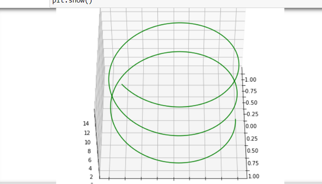
Example 2: In this example, we will plot a curve graph with an elevated angle of 120 degrees and a horizontal angle of 30 degrees.

Python3

from mpl_toolkits import mplot3d
import numpy as np
import matplotlib.pyplot as plt

fig = plt.figure(figsize = (8, 8))
ax = plt.axes(projection = '3d')

# Data for a three-dimensional line
z = np.linspace(0, 15, 1000)
x = np.sin(z)
y = np.cos(z)
ax.plot3D(x, y, z, 'green')

ax.view_init(120, 30)

plt.show()

Output:

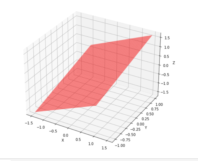
Example 3: In this example, we will plot a rectangular plate graph with an angle view of 50 degrees.

Python3

import numpy as np
from matplotlib import pyplot as plt
from mpl_toolkits.mplot3d import Axes3D
from math import sin, cos

fig = plt.figure(figsize = (8,8))
ax = fig.add_subplot(111, projection = '3d')

#creating Datasheet
y = np.linspace(-1, 1, 200)
x = np.linspace(-1, 1, 200)
x,y = np.meshgrid(x, y)

#set z values
z = x + y

# rotate the samples by changing the value of 'a'
a = 50

t = np.transpose(np.array([x, y, z]), ( 1, 2, 0))

m = [[cos(a), 0, sin(a)],[0, 1, 0],
     [-sin(a), 0, cos(a)]]

X,Y,Z = np.transpose(np.dot(t, m), (2, 0, 1))

#label axes
ax.set_xlabel('X')
ax.set_ylabel('Y')
ax.set_zlabel('Z')

#plot figure
ax.plot_surface(X,Y,Z, alpha = 0.5,
                color = 'red')

plt.show()

Output: