How to Calculate Autocorrelation in Python?
Last Updated :
17 Jan, 2022
Correlation generally determines the relationship between two variables. Correlation is calculated between the variable and itself at previous time steps, such a correlation is called Autocorrelation.
Method 1 : Using lagplot()
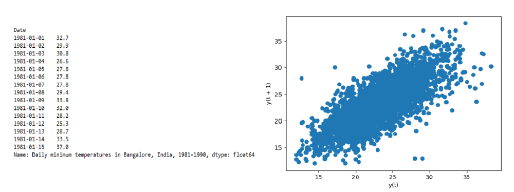
The daily minimum temperatures dataset is used for this example. As the first step, the autocorrelation can be quickly checked using lagplot() function provided by pandas.
Syntax:
pd.plotting.lag_plot(data, lag=1)
where,
- data is the input dataframe
- lag specifies integer to get the lags
Data Used: daily-minimum-temperatures-in-blr
Python3
import pandas as pd
data = pd.read_csv("daily-minimum-temperatures-in-blr.csv",
header=0, index_col=0, parse_dates=True,
squeeze=True)
data.head(15)
pd.plotting.lag_plot(data, lag=1)
|
Output:
Method 2: Creating lagged variables at different time steps
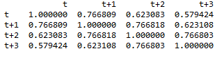
As we are aware of the fact that, the values of the observation at the current and previous time steps are significant in predicting the future step, let’s create lagged variables at different timesteps say, t+1, t+2, t+3. This is done using pandas.concat() and shift() function. Shift function shifts the timestep by a specified value and the Concat function joins the lagged variables at different timesteps as shown below.
Use pandas.corr() function on the new dataframe to calculate the correlation matrix.
Syntax:
pandas.DataFrame.corr(method = 'pearson')
where, method – pearson which is for calculating the standard correlation coefficient
Example:
Python3
data = pd.read_csv("daily-minimum-temperatures-in-blr.csv",
header=0, index_col=0, parse_dates=True,
squeeze=True)
values = pd.DataFrame(data.values)
dataframe = pd.concat([values.shift(3), values.shift(2),
values.shift(1), values], axis=1)
dataframe.columns = ['t', 't+1', 't+2', 't+3']
result = dataframe.corr()
print(result)
|
Output:
Method 3: Using plot_acf()
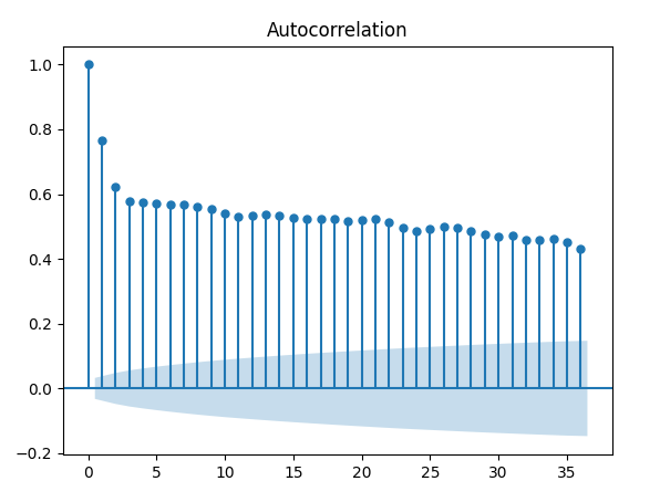
A plot of the autocorrelation of a time series by lag is called the AutoCorrelation Function (ACF). Such a plot is also called a correlogram. A correlogram plots the correlation of all possible timesteps. The lagged variables with the highest correlation can be considered for modeling. Below is an example of calculating and plotting the autocorrelation plot for the dataset chosen.
Statsmodel library provides a function called plot_acf() for this purpose.
Syntax:
statsmodels.graphics.tsaplots.plot_acf(x,lags,alpha)
where,
- x – An array of time-series values
- lags – An int or array of lag values, used on the horizontal axis. Uses np.arange(lags) when lags is an int.
- alpha – If a number is given, the confidence intervals for the given level are returned. For instance, if alpha=.05, 95 % confidence intervals are returned where the standard deviation is computed according to Bartlett’s formula. If None, no confidence intervals are plotted.
Example:
Python3
import pandas as pd
from statsmodels.graphics.tsaplots import plot_acf
data = pd.read_csv("daily-minimum-temperatures-in-blr.csv",
header=0, index_col=0, parse_dates=True,
squeeze=True)
plot_acf(data)
|
Output:
Share your thoughts in the comments
Please Login to comment...