How to Auto Update a Chart After Entering New Data in Excel

When you build a chart in Excel, it’s challenging to keep it up to date, even if you subsequently add new data. Although you may manually alter the chart’s data range to reflect the new data, this can be time-consuming if your spreadsheet is constantly updated. Fortunately, there is a simpler approach. 

To save you time, Simply prepare your source data as a table before creating a chart based on it. When you add new data below the table, it will be reflected in both the table and the chart, keeping everything consistent and up to date. 

In this article, we will discuss how to auto-update a chart in Excel after entering any new data into it. Users must be familiar with Excel and the type of charts possible to make in Excel.

Auto Update a Chart After Entering New Data in Excel

Updating a chart after entering data can be done in two ways:

1. Using tables

2. Using dynamic formula.

Example

This is the primary dataset that will be used here. I will manipulate this Dataset by adding or removing rows/columns or values.

Auto-Update a Chart after Entering New Data in Excel using Tables 

If we convert the above dataset into a Table then no matter what we add to it, the chart will be updated automatically.

Step 1: Select the entire dataset and click on Insert on the top of the ribbon and then select Table. The following dialog box opens.

Remember to check: My table has a headers option is checked. Headers are the column names such as Student Name, DSA, OS, etc. Now our dataset is a Table, now whenever we add any new values to the table like rows or columns or add columns our plot will get updated.

Step 2: Now select the entire table and from Insert click on any type of chart the user like. Here Plot is generated with the default dataset.  

Step 3: Then add a new row or column or change any value and see the plot which automatically changes. After Adding a new Row with some values.

Added Raj row with different values and the chart gets updated accordingly

Video Output of the Process

Auto-Update a Chart after Entering new data in Excel Using the Dynamic Formula

Using Dynamic formula is another way of auto-update a chart after entering new data in Excel. If the user doesn’t want to change the table range then this dynamic formula comes in role. To use dynamic formula you have to insert a dataset in the sheet and create a chart. If you don’t know how to create a chart you can learn How to create a chart in Excel?

Let’s discuss the example :

Below is a dataset of students and their subject marks. 

 Follow the steps to create a dynamic formula.

Step 1:Firstly click on the defined name in the formula and create a dynamic formula for each column. 

Step 2: In the New Name dialog box, fill Name as StudentName, scope as a current worksheet, and write a dynamic formula in refers to column i.e,

=OFFSET($A$2,0,0,COUNTA($A:$A)-1)  then click “OK”

Things to know: In the above formula the OFFSET() is the function that refers to the first data point and COUNTA refers to the column of the data.

Repeat the above process and create a dynamic formula for each series using the following range names and formulas. 

1. Dynamic formula for column B(DSA): =OFFSET($B$2,0,0,COUNTA($B:$B)-1)
2. Dynamic formula for column C(OS): =OFFSET($C$2,0,0,COUNTA($C:$C)-1)
3. Dynamic formula for column D(DBMS): =OFFSET($D$2,0,0,COUNTA($D:$D)-1)

Step 3: Now right-click on any of the bars and choose “Select data”.

Step 4: A “Select data source” dialog box will appear. Now In the Legend Entries (Series) section. 

• Select DSA and then click the edit button.

Step 5: Edit series will pop up, type “=Sheet2!DSA” in the series value section as shown below.

Repeat the same step for the other series also to update the other series as mentioned below:

1. OS – “=Sheet1!OS
2. DBMS -“Sheet1!DBMS  

Step 6: Now, On the right side of the Select data source, click Edit under Horizontal (Category) Axis Labels. 

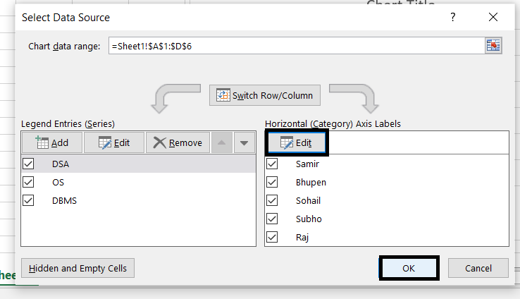
Step 7: A dialog box of Axis label will pop up, enter “Sheet1! Student_name” and click “OK”.

FAQs

How can I Update a Chart after entering new data in Excel?

This can be done in two ways:

Using tables 

Using dynamic formula

How often the chart will update with the new data?

The chart will reflect the changes immediately as you enter the data into the table (input the data in the specified region).

Can the Chart be updated from another Worksheet?

Yes, the chart can be updated with the data from another worksheet. When defining a named range or specifying the chart’s data range, include the worksheet name followed by an exclamation mark (!). 

Example:  If your data is on another worksheet (Sheet3) and the named range is “Chart”, Then you will have to use “=Sheet3!chart” as the chart data range.

What if I want to update the chart Automatically when new data is added to multiple columns?

To update the chart automatically when new data is added to multiple columns, you can define named ranges for each column and use those named ranges as the data source for the chart. Then whenever new data is added to any of the named ranges, the chart will update accordingly.