How to add White Gaussian Noise to Signal using MATLAB ?

In this article, we are going to discuss the addition of “White Gaussian Noise” to signals like sine, cosine, and square wave using MATLAB. The white Gaussian noise can be added to the signals using MATLAB/GNU-Octave inbuilt function awgn(). Here, “AWGN” stands for “Additive White Gaussian Noise”.

AWGN is a very basic noise model commonly used in the communication system, signal processing, and information theory to imitate the effect of random processes that occur in nature. 

We normally have different syntaxes for awgn() function depending on the number and type of parameters passed to it. But here, we will study only two syntaxes of it which are most commonly used in the communication system and signal processing.

Syntax:

awgn(input_signal, snr)

This syntax will add the white Gaussian noise to the passed input_signal and maintains the passed SNR (signal to noise ratio) in dB. By default this syntax considers the power of the input_signal as 0 dBW (decibel watt).

awgn(input_signal, snr, signal_power)

This syntax will do the same thing as the first one but the only difference is, here the power of the input_signal is not considered as zero rather it has to be passed as one of the arguments along with the input_signal and snr.

Note: Signal power can be passed as “measured” or some scalar value to set the signal level of the input_signal, according to which the appropriate noise level is determined based on the value of snr.

Stepwise Implementation

Let’s understand the implementation with the help of an example where we will add the gaussian white noise to the sine waves.

Step 1: Define the required parameters

Matlab

% sampling frequency
fs = 1000;

% time sampling with step
% size = 0.001 (1/fs)
t = 0:1/fs:1;

% frequency of input signal
f = 20;

% SNR to be maintained
snr = 10;

Step 2: Define the input signal and plot 

Matlab

% input message signal (sine wave)
% generates a sine wave of frequency f
st = sin(2 * pi * f * t);

% plot the input signal (sine wave)
% 'b' gives blue colour plot
plot(t, st, 'b', 'Linewidth', 2);
xlabel('Time');
ylabel('Amplitude');
title('Input Message Signal');
grid on;

Output:

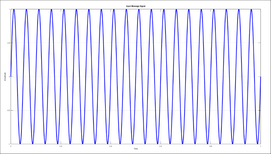
Input Signal (Sine Wave)

Step 3: Add white Gaussian noise to signal and plot

Matlab

% signal with white Gaussian noise
% adds White Gaussian Noise to the signal
st_nn = awgn(st, snr, 'measured');

% plot the noisy signal
% 'r' gives red colour plot
plot(t, st_nn, 'r', 'Linewidth', 2);
xlabel('Time');
ylabel('Amplitude');
title('Signal After Addition of Noise');
grid on;

Output:

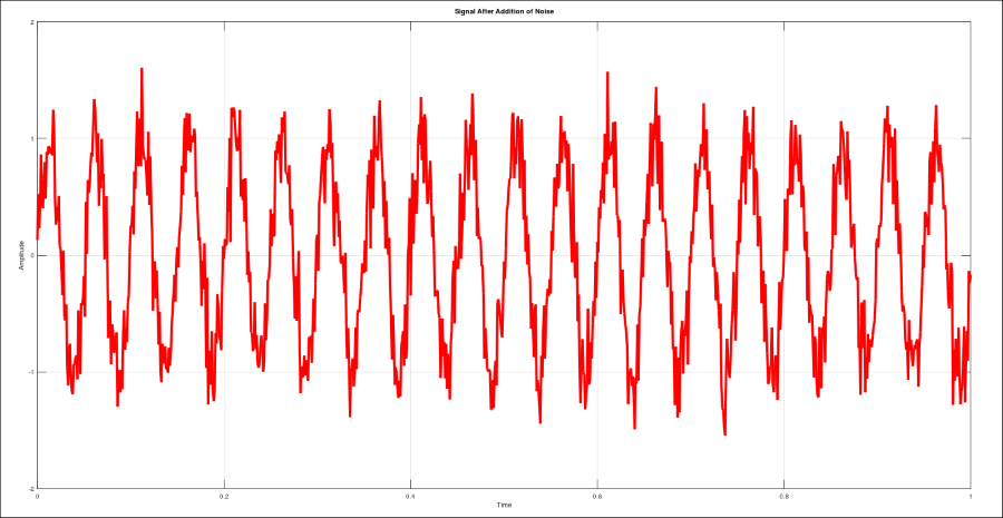
Noisy Signal (With white Gaussian noise)

Let’s see another example Addition of white Gaussian noise to square wave. We have to follow the same three steps as above to add the white Gaussian noise to the square wave. But this time we will plot both the input signal and the noisy signal simultaneously in the same figure to analyze the changes carefully.

Matlab

% sampling frequency
fs = 1000;

% time sampling with step size
% 0.001 (1/fs)
t = 0:1/fs:1;

% frequency of input signal
f = 10;

% SNR to be maintained
snr = 5;

% Input Message Signal
% generates a square wave of
% frequency f
st = square(2 * pi * f * t);
subplot(2,1,1);

% 'b' gives blue colour plot
plot(t,st,'b','Linewidth',2);
xlabel('Time'); ylabel('Amplitude');
title('Input Message Signal');
grid on;

% signal with white Gaussian
% noise adds White Gaussian
% Noise to the signal
st_nn = awgn(st,snr,'measured');

% gives a blue colour plot of
% square wave
subplot(2,1,2); plot(t, st, 'b', 'Linewidth', 2);

% puts the next graph on the
% same plot
hold on;

% gives a red colour plot of the
% AWGN noise
plot(t, st_nn, 'r');
xlabel('Time');
ylabel('Amplitude');
title('Signal After Addition of Noise');
grid on;
hold off;

Output:

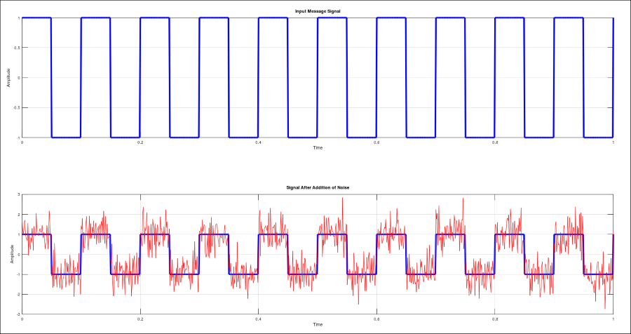
Output Plots