How to add image to ggplot2 in R ?

In this article, we will discuss how to insert or add an image into a plot using ggplot2 in R Programming Language.

The ggplot() method of this package is used to initialize a ggplot object. It can be used to declare the input data frame for a graphic and can also be used to specify the set of plot aesthetics. The ggplot() function is used to construct the initial plot object and is almost always followed by components to add to the plot. 

Syntax:

ggplot(data, mapping = aes())

Parameters : 

• data – The data frame used for data plotting
• mapping – Default list of aesthetic mappings to use for plot.

Method 1: Using patchwork package 

The “jpeg” package is used to provide an easy way to perform operations with JPEG images, that is, read, write and display bitmap images stored in the JPEG format.

Syntax:

install.packages(“jpeg”)

The readJPEG() method of this package is used to access an image from a JPEG file/content into a raster array. It reads a bitmap image into a native rasterImage. 

Syntax:

readJPEG(path, native = FALSE)

Parameters : 

• path –  The name of the JPEG file to access into the working space. 
• native – Indicator of the image representation. If TRUE then the result is a native raster representation.

Another package, “patchwork” allows arbitrarily complex composition of plots by providing mathematical operators for combining multiple plots. It is used for enhancement and descriptive plot construction and analysis. It is mainly intended for users of ggplot2 and ensures its proper alignment. 

Syntax:

install.packages(“patchwork”)

The inset_element() function of this package provides a way to create additional insets and gives you full control over the placement and orientation of these insets with respect to each other. The method marks the specified graphics as an inset to be added to the preceding plot.

Syntax:

inset_element( p, left, bottom, right, top)

Parameter:

• p – A grob, ggplot, patchwork, formula, raster, or nativeRaster object to be added as an inset to the plot.
• left, bottom, right, top – the coordinate positions for adding p. 

Example:

R

# loading the required libraries
library("jpeg")
library("ggplot2")
library("patchwork")

# defining the x coordinates
xpos <- 1:5

# defining the y coordinates
ypos <- xpos**2

data_frame = data.frame(xpos = xpos,
                        ypos = ypos)

print ("Data points")
print (data_frame)

# plotting the data
graph <- ggplot(data_frame, aes(xpos, ypos)) +
  geom_point()

# specifying the image path
path <- "/Users/mallikagupta/Desktop/GFG/gfg.jpeg"

# read the jpef file from device
img <- readJPEG(path, native = TRUE)

# adding image to graph
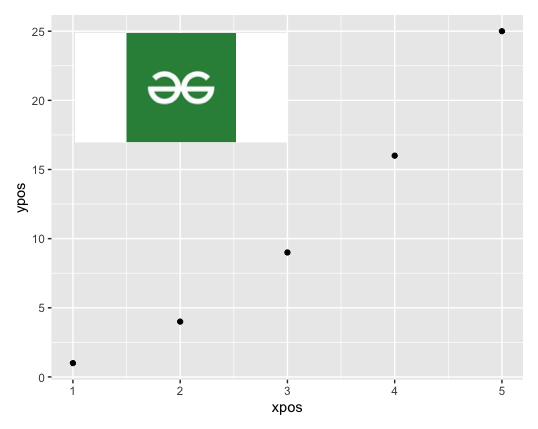
img_graph <- graph +
  inset_element(p = img,
                left = 0.05,
                bottom = 0.65,
                right = 0.5,
                top = 0.95)

# printing graph with image
print (img_graph)

Output

[1] "Data points" 
   xpos ypos 
1    1    1 
2    2    4 
3    3    9 
4    4   16 
5    5   25

Method 2: Using grid package

The grid package in R is concerned with graphical functions that are used for the creation of the ggplot2 plotting system.

Syntax:

install.packages(“grid”)

The rasterGrob() method in R is used to create a raster image graphical object into the working space. It takes as input the image path (either PNG or JPEG) as the first argument and converts it into a raster graphical image. 

Syntax:

rasterGrob (path, interpolate = TRUE)

The qplot() method in R is used to create a quick plot which can be used as a wrapper over various other methods of creating plots. It makes it easier to create complex graphics.

Syntax: 

qplot(x, y=NULL, data, geom=”auto”, xlim = c(NA, NA), ylim =c(NA, NA))

Parameters : 

• x, y – x and y coordinates
• data – data frame to be used
• geom – indicator of the geom to be used
• xlim, ylim – x and y axis limits

The annotation_custom() can be combined with the qplot() method which is a special geom intended for use as static annotations. The actual scales of the plots remain unmodified using this option. 

Syntax:

annotation_custom(grob, xmin = -Inf, xmax = Inf, ymin = -Inf, ymax = Inf)

Parameters : 

• g – The grob to display
• xlim, ylim – x and y axis limits

Example:

R

# loading the required libraries
library("jpeg")
library("ggplot2")
library("grid")

# defining the x coordinates
xpos <- 1:5

# defining the y coordinates
ypos <- xpos**2

data_frame = data.frame(xpos = xpos,
                        ypos = ypos)

print ("Data points")
print (data_frame)

# specifying the image path
path <- "/Users/mallikagupta/Desktop/GFG/gfg.jpeg"

# read the jpef file from device
img <- readJPEG(path, native = TRUE)

# converting to raster image
img <- rasterGrob(img, interpolate=TRUE)

# plotting the data
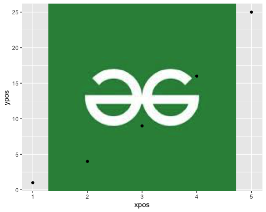
qplot(xpos, ypos, geom="blank") +
  annotation_custom(g, xmin=-Inf, xmax=Inf, ymin=-Inf, ymax=Inf) +
  geom_point()

Output

[1] "Data points"
  xpos ypos
1    1    1
2    2    4
3    3    9
4    4   16
5    5   25