How to add a frame to a seaborn heatmap figure in Python?

Difficulty Level : Easy
Last Updated : 03 Jan, 2021

A heatmap is a graphical representation of data where values are depicted by color. They make it easy to understand complex data at a glance. Heatmaps can be easily drawn using seaborn in python. In this article, we are going to add a frame to a seaborn heatmap figure in Python.

Syntax: seaborn.heatmap(data, *, vmin=None, vmax=None, cmap=None, center=None, annot_kws=None, linewidths=0, linecolor=’white’, cbar=True, **kwargs)
Important Parameters:
data: 2D dataset that can be coerced into an ndarray.
linewidths: Width of the lines that will divide each cell.
linecolor: Color of the lines that will divide each cell.
cbar: Whether to draw a colorbar.
All the parameters except data are optional.
Returns: An object of type matplotlib.axes._subplots.AxesSubplot

Create a heatmap

To draw the heatmap we will use the in-built data set of seaborn. Seaborn has many in-built data sets like titanic.csv, penguins.csv, flights.csv, exercise.csv. We can also make our data set it should just be a rectangular ndarray.

Python3

# Import libraries
import seaborn as sns
import matplotlib.pyplot as plt
  
# Preparing dataset
example = sns.load_dataset("flights")
example = example.pivot("month", "year",
                        "passengers")
  
# Creating plot
res = sns.heatmap(example)
  
# show plot
plt.show()

Output:

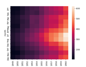
basic heatmap

There are two ways of drawing the frame around a heatmap:

Using axhline and axvline.
Using spines (more optimal)

Method 1: Using axhline and axvline

The Axes.axhline() and Axes.axvline() function in axes module of matplotlib library is used to add a horizontal and vertical line across the axis respectively.

We can draw two horizontal lines from y=0 and from y= number of rows in our dataset and it will draw a frame covering two sides of our heatmap. Then we can draw two vertical lines from x=0 and x=number of columns in our dataset and it will draw a frame covering the remaining two sides so our heatmap will have a complete frame.

Note: It is not an optimal way to draw a frame as when we increase the line width is does not consider when it is overlapping the heatmap.

Example 1.

Python3

# Import libraries
import seaborn as sns
import matplotlib.pyplot as plt
  
# Preparing dataset
example = sns.load_dataset("flights")
example = example.pivot("month", "year",
                        "passengers")
  
# Creating plot
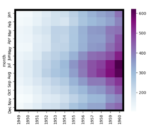
res = sns.heatmap(example, cmap = "BuPu")
  
# Drawing the frame
res.axhline(y = 0, color='k',linewidth = 10)
res.axhline(y = example.shape[1], color = 'k',
            linewidth = 10)
  
res.axvline(x = 0, color = 'k',
            linewidth = 10)
  
res.axvline(x = example.shape[0], 
            color = 'k', linewidth = 10)
  
# show plot
plt.show()

Output:

Example 2:

Python3

# Import libraries
import seaborn as sns
import matplotlib.pyplot as plt
import numpy as np
  
# Preparing dataset
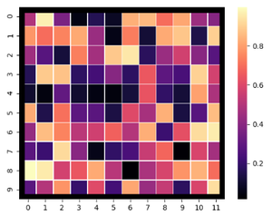
example = np.random.rand(10, 12)
  
# Creating plot
res = sns.heatmap(example, cmap = "magma", 
                  linewidths = 0.5)
  
# Drawing the frame
res.axhline(y = 0, color = 'k', 
            linewidth = 15)
  
res.axhline(y = 10, color = 'k',
            linewidth = 15)
  
res.axvline(x = 0, color = 'k',
            linewidth = 15)
  
res.axvline(x = 12, color = 'k',
            linewidth = 15)
# show plot
plt.show()

Output:

Method 2: Using spines

Spines are the lines connecting the axis tick marks and noting the boundaries of the data area. They can be placed at arbitrary positions.

Example 1:

width of the line can be changed using the set_linewidth parameter which accepts a float value as an argument.

Python3

# Import libraries
import seaborn as sns
import matplotlib.pyplot as plt
  
# Preparing dataset
example = sns.load_dataset("flights")
example = example.pivot("month", "year", 
                        "passengers")
  
# Creating plot
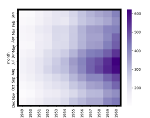
res = sns.heatmap(example, cmap = "Purples")
  
# Drawing the frame
for _, spine in res.spines.items():
    spine.set_visible(True)
    spine.set_linewidth(5)
  
# show plot
plt.show()

Output:

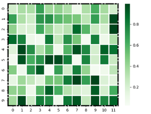
Example 2:

We can specify the style of the frame using the set_linestyle parameter of the spine(solid, dashed, dashdot, dotted).

Python3

# Import libraries
import seaborn as sns
import matplotlib.pyplot as plt
import numpy as np
  
# Preparing dataset
example = np.random.rand(10, 12)
  
# Creating plot
res = sns.heatmap(example, cmap = "Greens",
                  linewidths = 2,
                  linecolor = "white")
  
# Drawing the frame
for _, spine in res.spines.items():
    spine.set_visible(True)
    spine.set_linewidth(3)
    spine.set_linestyle("dashdot")
  
# show plot
plt.show()