Excel HLOOKUP Function with Formula Examples

Excel has several functions to search data from a table. HLOOKUP() function is one of them. The ‘H’ in the HLOOKUP() function stands for ‘horizontal’. This function generally helps to find a value from a row of an array or table. For this function to work the lookup value must be in the first row of the table or array. HLOOKUP() moves downward and searches for the required output. Like VLOOKUP() this function also supports exact and approximate matches. 

Try using the new XLOOKUP function, An improved version of HLOOKUP that works in any direction and gives the exact match by default. 

What is HLOOKUP in Excel?

HLOOKUP is a function that is used to search for a value in the topmost row of a table, and then return a corresponding value in the same column from a row you specify but this lookup function is not very popular because most of the tables that we deal with are vertical hence this function is not very popular.

What is the Difference between HLOOKUP and VLOOKUP

In Excel, you have three lookup functions: XLOOKUP, HLOOKUP, and VLOOKUP. They each have specific ways of searching for and retrieving data from tables:

VLOOKUP (Vertical Lookup)

• It looks for a value in the leftmost (first) column of a table.
• Then, it retrieves a corresponding value from the same row in a specified column to the right.
• VLOOKUP is best for tables organized vertically (columns).
• To use it, you need to specify the column index number for the desired value.
• It’s limited to vertical lookups.

HLOOKUP (Horizontal Lookup)

• HLOOKUP searches for a value in the topmost (first) row of a table.
• It retrieves a corresponding value from the same column in a specified row below.
• HLOOKUP is suitable for tables organized horizontally (rows).
• Its syntax is similar to VLOOKUP but requires specifying the row index number.
• HLOOKUP can only perform horizontal lookups.
• In essence, VLOOKUP and HLOOKUP differ in their search directions. VLOOKUP searches up and down columns, while HLOOKUP searches left and right across rows. Your choice between them depends on your data’s organization and whether you need vertical or horizontal lookups.

When to use HLOOKUP in Excel

HLOOKUP() function is used when the user tries to find a value in a table by matching a lookup value in the first row of the table. Generally, the user wants an exact match. This function searches for a value horizontally as its name means.

Syntax

=HLOOKUP(lookup_value, table_array, row_index_num, [range_lookup])

Here, the [range_lookup] argument is optional.

In simple language,

=HLOOKUP(search for this value, in this table, returns a value from this row, [return an  approximate or exact value])

So, HLOOKUP() takes four arguments as input and returns the desired output.

Arguments

• lookup_value (Required): This is the value( maybe a value, a reference, or a text string) that the HLOOKUP() function tries to match in the first row of the table. This argument must be provided by the user.
• table_array (Required): This is the table or the reference of a table where the HLOOKUP() function tries to match the lookup_value and searches for the output. Also, this argument must be provided by the user.
• row_index_num (Required): This is the row number where the HLOOKUP() function searches for the output. This argument should be provided by the user. This value cannot be less than 1 or greater than the number of rows in the table_array. This function shows an error(#VALUE! Or #REF!) in both cases.
• [range_lookup] (Optional): This is an optional argument. It contains a logical value(TRUE or FALSE) by which HLOOKUP() can understand if the user wants an approximate or an exact match. This value is TRUE by default(If the user does not provide any value). TRUE denotes an approximate match and FALSE denotes an exact match.

Note: If the [range_lookup] value is FALSE and the user wants to partially match a text, wildcards(‘*’ or ‘?’) can be used. An asterisk matches a sequence and a question mark matches a single character. And this function is not case-sensitive.

Return Value: HLOOKUP() first matches the lookup value in the first column of the table and then moves downward to search for the output value. After all, it returns that output value.

Example of HLOOKUP function

The list below is taken for the example:

Product Name	Computer	Television	Printer	Keyboard	Speakers
In stock	22	18	17	16	15
Sold	2	5	8	10	11
Price per item	30000	18000	15000	800	500

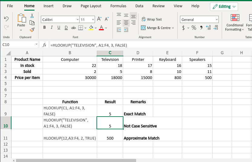
In the above list HLOOKUP() function is applied:

HLOOKUP function	Result	Description
HLOOKUP(C1, A1:F4, 3, FALSE)	5	Here the user wants an exact match for the lookup value “Television”  and wants the output from the 3rd row.
HLOOKUP(“TELEVISION”, A1:F4, 3, FALSE)	5	This result proves that the HLOOKUP function is not case-sensitive.
HLOOKUP(12,A3:F4, 2, TRUE)	500	Here the user wants an approximate match for the lookup value 12 and wants  the output from the 2nd row of the table array.  If TRUE is omitted in this function it will return the same result.

Output:

Output Screenshot

How to do HLOOKUP  from Another Workbook and Worksheet in Excel

Giving an external reference to our HLOOKUP formula. 

To extract our matching data from another worksheet, mention the sheet name followed by an exclamation mark. 

For example, we have two worksheets. Named Sheet1 And Sheet2, We want our data from Sheet 2 to Sheet 1. We have to apply the formula of HLOOKUP by giving the reference of sheet 2. 

Formula used is =HLOOKUP(B1,Sheet2!A1:F2,2,False) . Drag the formula to other cells to copy the formula of HLOOKUP.

Data from sheet 2 (sold) is copied from sheet 2 to sheet 1. 

Excel HLOOKUP with Partial Match (wildcard characters)

ust like VLOOKUP, you can use wildcard characters in Excel’s HLOOKUP function when searching for data:

The question mark (?) matches any single character.

The asterisk (*) matches any sequence of characters.

Note: To make a wildcard HLOOKUP formula work correctly, ensure that the “range_lookup” argument is set to FALSE.

If your “table_array” contains multiple values that match the wildcard criteria, the formula will return the first value it finds.

Absolute and Relative Cell Reference

This concept comes in use when you copy the formula to multiple cells. If you want to know more about cell reference then click here.

Use of Relative and Absolute cell reference:

• Table_array should be fixed by using absolute cell reference with dollar sign($) For example: $B$1:$1$2.
• The lookup Reference is relative or mixed depending on your use.

Below is the formula that is used to take data from another worksheet.

=HLOOKUP(B$1,Sheet2!$A$1:$F$2,2,False)

We have used Absolute cell reference ($A$2:$F$2) in table_array that is because it should remain the same when we are copying the formula to other cells. 

We have used Mixed cell reference for lookup value (B$1) because our data is present in relative column and absolute row and our lookup values are present in the same row (sold) but in different columns (B to F).

Note: Reference should change based on a relative position of a cell where formula is copied.

Things to Remember

• It is case – insensitive lookup. It will consider “sold” and “SOLD” as same.
• The ‘Lookup_value’ should be the topmost row of the ‘table_array’ while using HLOOKUP. We have to use another formula to look for a value somewhere else.
• HLOOKUP supports the wildcards characters such as ‘*’ or ‘?’ in the ‘lookup_value’ argument (only if ‘lookuo_value ‘ is text).

FAQs on the HLOOKUP Function 

Q1: What if the HLOOKUP can’t find the Lookup value?

Answer

 If HLOOKUP can’t find the lookup value and range_lookup is TRUE, it will consider the largest value that is less than lookup_value.

Q2: What if the LOOKUP value is smaller than the smallest value in the first row of the table array?

Answer:

If the LOOKUP value is smaller than smallest value in the first row of the table_array, HLOOKUP returns the error value.

Q3: What is the difference between VLOOKUP and HLOOKUP?

Answer:

Both of the function search for lookup value. The difference is that how it is being used. 

Firstly the name itself is different, V in VLOOKUP is stands for Vertical search that is in a column or to the left of the data that you want to find.

And the H in HLOOKUP function stands for horizontal search, It searches the value at the top most row of the table and returns a value located at the specified number of rows down in the same column.

Q4: What does this formula mean by “HLOOKUP(10,{1,2,3:”a”,”b”,c”,”d”},2, true)?

Answer:

This formula indicates that Lookup the value 10 in the three row array constant and return the value form row 2 in the third column. There are three rows of values in the array constant separated by a semicolon (;) because “c” is found in the row 2 and in the same column as 3, “c” is returned.