Histogram Equalization using R language

Histogram equalization is a technique for adjusting image intensities to enhance contrast. To enhance the image’s contrast, it spreads out the most frequent pixel intensity values or stretches out the intensity range of the image. By accomplishing this, histogram equalization allows the image’s areas with lower contrast to gain a higher contrast.

Histogram Equalization can be used when you have images that look washed out because they do not have sufficient contrast. In such photographs, the light and dark areas blend together creating a flatter image that lacks highlights and shadows. To overcome this problem, we can use histogram equalization.

R programming language supports sub-systems to deal with this. This article is aimed at equalizing a histogram using R Programming language.

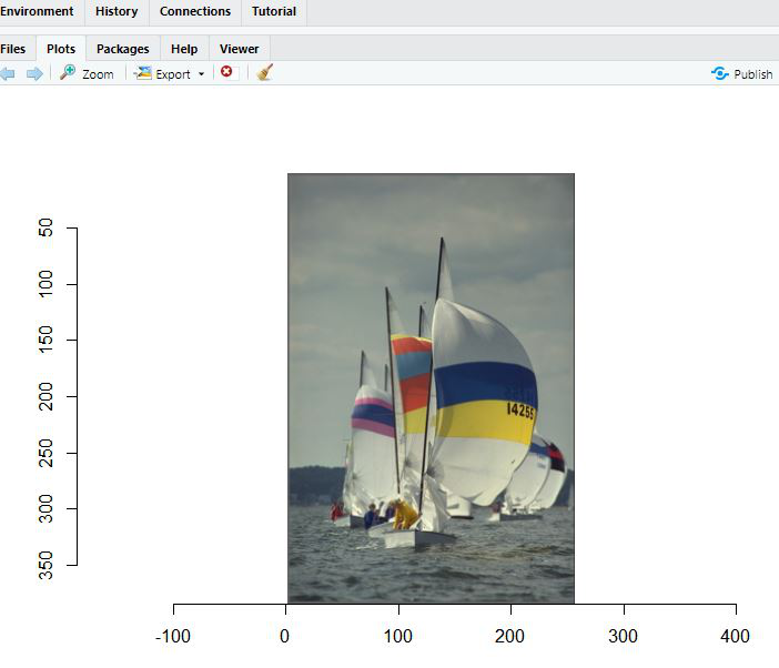
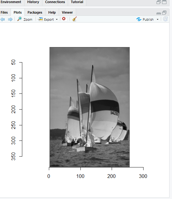
First Install imager package in Rstudio. Imager is an image/video processing package for R, based on CImg. (The image used here is already in the package ). Then we will read the image and grayscale it. To grayscale it only simply pass the loaded image to grayscale() function as an argument.

Syntax:

grayscale(image)

 The plot () function is used for plotting the images.

Example:

R

library(imager)

# original image
plot(boats)

boats.g <- grayscale(boats)

# grayscaled image
plot(boats.g)

Output:

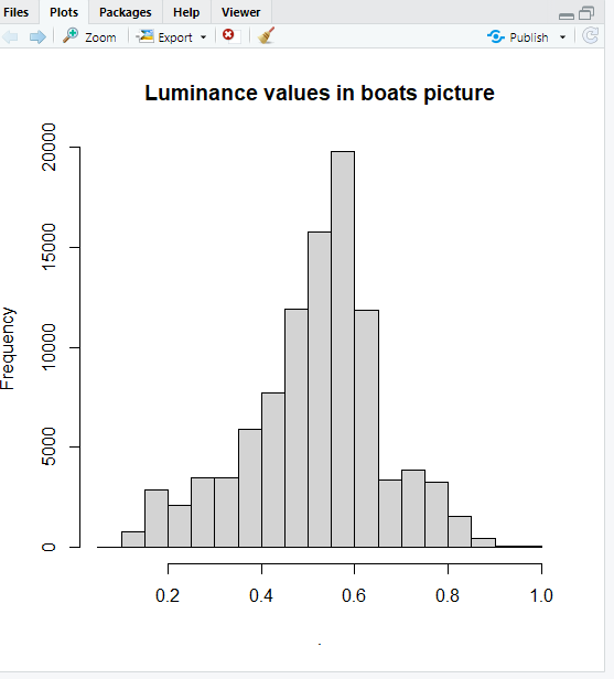
Now to see the luminance value in the image, use hist() before equalization. The main attribute is used to give the title to histogram.

Syntax:

grayscale(image) %>% hist(main=”heading”)

Example:

R

library(imager)

grayscale(boats) %>% hist(main="Luminance values in boats picture")

Output:

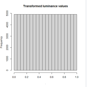
We will grayscale the image and calculate the cumulative distribution of image pixels using ecdf() function. It will also transform the luminance value in histogram, and will make the grayscaled image equalize. 

Then the as.cimg() is used to convert a data into an image. The dim attribute is basically the dimensions of the image.

Syntax:

f <- ecdf(image.g)

f(image.g) %>% hist(main=”Heading”)

f(image.g) %>% as.cimg(dim=dim(image.g)) %>% plot(main=”heading”)

# Hist. equalization for grayscale

hist.eq <- function(im) as.cimg(ecdf(im)(im),dim=dim(im))

Example:

R

library(imager)

f <- ecdf(boats.g)
f(boats.g) %>% hist(main="Transformed luminance values")
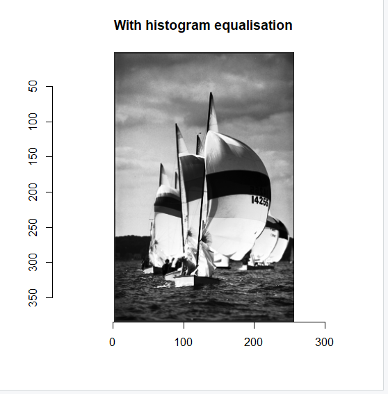
f(boats.g) %>% as.cimg(dim=dim(boats.g)) %>% plot(
  main="With histogram equalisation")

# Hist. equalisation for grayscale
hist.eq <- function(im) as.cimg(ecdf(im)(im),dim=dim(im))

Output:

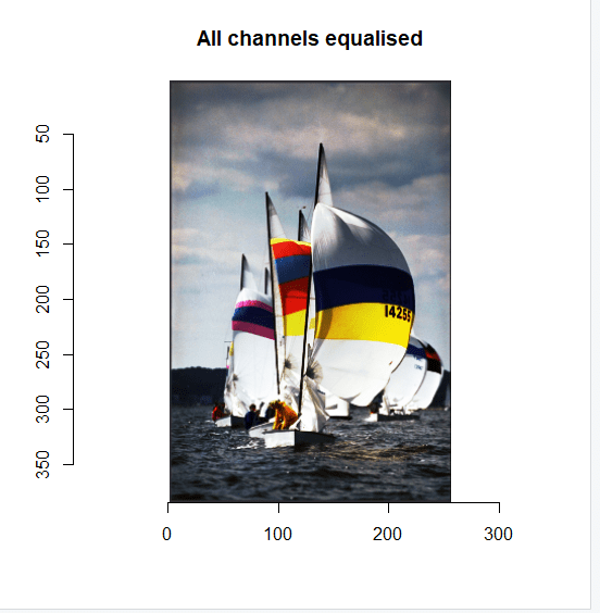
Now we will split the image across the color channels and equalize the colored image also. The imsplit() function is used to split the image across color channels and “c” is the axis passed. The map_il() function will map the hist.eq variable with each of the splitted color channeled images and will make sure that the output should be an image. The imappend() function will recombine the splitted images along the “c” axis and the plot() function will plot the equalized image.

Syntax:

#Split across colour channels,

cn <- imsplit(image,”c”)

#we now have a list of images

cn 

#run hist.eq on each

cn.eq <- map_il(cn,hist.eq) 

#recombine and plot

imappend(cn.eq,”c”) %>% plot(main=”Heading”) 

Example:

R

library(imager)

# Split across colour channels,
cn <- imsplit(boats,"c")

# we now have a list of images
cn

# run hist.eq on each
cn.eq <- map_il(cn,hist.eq)

# recombine and plot
imappend(cn.eq,"c") %>% plot(main="All channels equalised")

Output: