Hidden Markov Model in Machine learning

A statistical model called a Hidden Markov Model (HMM) is used to describe systems with changing unobservable states over time. It is predicated on the idea that there is an underlying process with concealed states, each of which has a known result. Probabilities for switching between concealed states and emitting observable symbols are defined by the model.

Because of their superior ability to capture uncertainty and temporal dependencies, HMMs are used in a wide range of industries, including finance, bioinformatics, and speech recognition. HMMs are useful for modelling dynamic systems and forecasting future states based on sequences that have been seen because of their flexibility.

Hidden Markov Model in Machine Learning

The hidden Markov Model (HMM) is a statistical model that is used to describe the probabilistic relationship between a sequence of observations and a sequence of hidden states. It is often used in situations where the underlying system or process that generates the observations is unknown or hidden, hence it has the name “Hidden Markov Model.” 

It is used to predict future observations or classify sequences, based on the underlying hidden process that generates the data.

An HMM consists of two types of variables: hidden states and observations.

• The hidden states are the underlying variables that generate the observed data, but they are not directly observable.
• The observations are the variables that are measured and observed. 

The relationship between the hidden states and the observations is modeled using a probability distribution. The Hidden Markov Model (HMM) is the relationship between the hidden states and the observations using two sets of probabilities: the transition probabilities and the emission probabilities. 

• The transition probabilities describe the probability of transitioning from one hidden state to another.
• The emission probabilities describe the probability of observing an output given a hidden state.

Hidden Markov Model  Algorithm

The Hidden Markov Model (HMM) algorithm can be implemented using the following steps:

Step 1: Define the state space and observation space

• The state space is the set of all possible hidden states, and the observation space is the set of all possible observations.

Step 2: Define the initial state distribution

• This is the probability distribution over the initial state.

Step 3: Define the state transition probabilities

•  These are the probabilities of transitioning from one state to another. This forms the transition matrix, which describes the probability of moving from one state to another.

Step 4: Define the observation likelihoods: 

• These are the probabilities of generating each observation from each state. This forms the emission matrix, which describes the probability of generating each observation from each state.

Step 5: Train the model

• The parameters of the state transition probabilities and the observation likelihoods are estimated using the Baum-Welch algorithm, or the forward-backward algorithm. This is done by iteratively updating the parameters until convergence.

Step 6: Decode the most likely sequence of hidden states

• Given the observed data, the Viterbi algorithm is used to compute the most likely sequence of hidden states. This can be used to predict future observations, classify sequences, or detect patterns in sequential data.

Step 7: Evaluate the model

• The performance of the HMM can be evaluated using various metrics, such as accuracy, precision, recall, or F1 score.

To summarise, the HMM algorithm involves defining the state space, observation space, and the parameters of the state transition probabilities and observation likelihoods, training the model using the Baum-Welch algorithm or the forward-backward algorithm, decoding the most likely sequence of hidden states using the Viterbi algorithm, and evaluating the performance of the model.

Implementation in Python

Key steps in the Python implementation of a simple Hidden Markov Model (HMM) using the hmmlearn library.

Example 1. Predicting the weather

Problem statement: Given the historical data on weather conditions, the task is to predict the weather for the next day based on the current day’s weather.

Step 1: Import the required libraries

The code imports the NumPy,matplotlib, seaborn, and the hmmlearn library.

Python3

# import the necessary libraries
import numpy as np
import matplotlib.pyplot as plt
import seaborn as sns
from hmmlearn import hmm

Step 2: Define the model parameters

In this example, The state space is defined as a state which is a list of two possible weather conditions: “Sunny” and “Rainy”. The observation space is defined as observations which is a list of two possible observations: “Dry” and “Wet”. The number of hidden states and the number of observations are defined as constants. 

Python3

# Define the state space
states = ["Sunny", "Rainy"]
n_states = len(states)
print('Number of hidden states :',n_states)
# Define the observation space
observations = ["Dry", "Wet"]
n_observations = len(observations)
print('Number of observations  :',n_observations)

Output:

Number of hidden states : 2
Number of observations  : 2

The start probabilities, transition probabilities, and emission probabilities are defined as arrays. The start probabilities represent the probabilities of starting in each of the hidden states, the transition probabilities represent the probabilities of transitioning from one hidden state to another, and the emission probabilities represent the probabilities of observing each of the outputs given a hidden state.

The initial state distribution is defined as state_probability, which is an array of probabilities that represent the probability of the first state being “Sunny” or “Rainy”. The state transition probabilities are defined as transition_probability, which is a 2×2 array representing the probability of transitioning from one state to another. The observation likelihoods are defined as emission_probability, which is a 2×2 array representing the probability of generating each observation from each state.

Python3

# Define the initial state distribution
state_probability = np.array([0.6, 0.4])
print("State probability: ", state_probability)

# Define the state transition probabilities
transition_probability = np.array([[0.7, 0.3],
                                   [0.3, 0.7]])
print("\nTransition probability:\n", transition_probability)
# Define the observation likelihoods
emission_probability= np.array([[0.9, 0.1],
                                 [0.2, 0.8]])
print("\nEmission probability:\n", emission_probability)

Output:

State probability:  [0.6 0.4]
Transition probability:
 [[0.7 0.3]
 [0.3 0.7]]
Emission probability:
 [[0.9 0.1]
 [0.2 0.8]]

Step 3: Create an instance of the HMM model and Set the model parameters

The HMM model is defined using the hmm.CategoricalHMM class from the hmmlearn library. An instance of the CategoricalHMM class is created with the number of hidden states set to n_hidden_states and the parameters of the model are set using the startprob_, transmat_, and emissionprob_ attributes to the state probabilities, transition probabilities, and emission probabilities respectively.

Python3

model = hmm.CategoricalHMM(n_components=n_states)
model.startprob_ = state_probability
model.transmat_ = transition_probability
model.emissionprob_ = emission_probability

Step 4: Define an observation sequence

A sequence of observations is defined as a one-dimensional NumPy array.

The observed data is defined as observations_sequence which is a sequence of integers, representing the corresponding observation in the observations list.

Python3

# Define the sequence of observations
observations_sequence = np.array([0, 1, 0, 1, 0, 0]).reshape(-1, 1)
observations_sequence

Output:

array([[0],
       [1],
       [0],
       [1],
       [0],
       [0]])

Step 5: Predict the most likely sequence of hidden states

 The most likely sequence of hidden states is computed using the prediction method of the HMM model.

Python3

# Predict the most likely sequence of hidden states
hidden_states = model.predict(observations_sequence)
print("Most likely hidden states:", hidden_states)

Output:

Most likely hidden states: [0 1 1 1 0 0]

Step 6: Decode the observation sequence

The Viterbi algorithm is used to calculate the most likely sequence of hidden states that generated the observations using the decode method of the model. The method returns the log probability of the most likely sequence of hidden states and the sequence of hidden states itself.

Python3

log_probability, hidden_states = model.decode(observations_sequence,
                                              lengths = len(observations_sequence),
                                              algorithm ='viterbi' )

print('Log Probability :',log_probability)
print("Most likely hidden states:", hidden_states)

Output:

Log Probability : -6.360602626270058
Most likely hidden states: [0 1 1 1 0 0]

This is a simple algo of how to implement a basic HMM and use it to decode an observation sequence. The hmmlearn library provides a more advanced and flexible implementation of HMMs with additional functionality such as parameter estimation and training.

Step 7: Plot the results

Python3

# Plot the results
sns.set_style("whitegrid")
plt.plot(hidden_states, '-o', label="Hidden State")
plt.xlabel('Time step')
plt.ylabel('Most Likely Hidden State')
plt.title("Sunny or Rainy")
plt.legend()
plt.show()

Output:

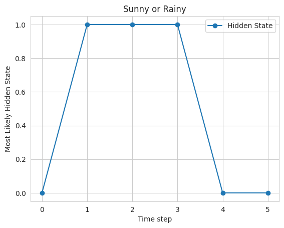
Sunny or Rainy

Finally, the results are plotted using the matplotlib library, where the x-axis represents the time steps, and the y-axis represents the hidden state. The plot shows that the model predicts that the weather is mostly sunny, with a few rainy days mixed in.

Example 2: Speech recognition

Problem statement: Given a dataset of audio recordings, the task is to recognize the words spoken in the recordings.

In this example, the state space is defined as states, which is a list of 4 possible states representing silence or the presence of one of 3 different words. The observation space is defined as observations, which is a list of 2 possible observations, representing the volume of the speech. The initial state distribution is defined as start_probability, which is an array of probabilities of length 4 representing the probability of each state being the initial state.

The state transition probabilities are defined as transition_probability, which is a 4×4 matrix representing the probability of transitioning from one state to another. The observation likelihoods are defined as emission_probability, which is a 4×2 matrix representing the probability of emitting an observation for each state.

The model is defined using the MultinomialHMM class from hmmlearn library and is fit using the startprob_, transmat_, and emissionprob_ attributes. The sequence of observations is defined as observations_sequence and is an array of length 8, representing the volume of the speech in 8 different time steps.

The predict method of the model object is used to predict the most likely hidden states, given the observations. The result is stored in the hidden_states variable, which is an array of length 8, representing the most likely state for each time step.

Python3

import numpy as np
import matplotlib.pyplot as plt
import seaborn as sns
from hmmlearn import hmm

# Define the state space
states = ["Silence", "Word1", "Word2", "Word3"]
n_states = len(states)

# Define the observation space
observations = ["Loud", "Soft"]
n_observations = len(observations)

# Define the initial state distribution
start_probability = np.array([0.8, 0.1, 0.1, 0.0])

# Define the state transition probabilities
transition_probability = np.array([[0.7, 0.2, 0.1, 0.0],
                                    [0.0, 0.6, 0.4, 0.0],
                                    [0.0, 0.0, 0.6, 0.4],
                                    [0.0, 0.0, 0.0, 1.0]])

# Define the observation likelihoods
emission_probability = np.array([[0.7, 0.3],
                                  [0.4, 0.6],
                                  [0.6, 0.4],
                                  [0.3, 0.7]])

# Fit the model
model = hmm.CategoricalHMM(n_components=n_states)
model.startprob_ = start_probability
model.transmat_ = transition_probability
model.emissionprob_ = emission_probability

# Define the sequence of observations
observations_sequence = np.array([0, 1, 0, 0, 1, 1, 0, 1]).reshape(-1, 1)

# Predict the most likely hidden states
hidden_states = model.predict(observations_sequence)
print("Most likely hidden states:", hidden_states)

# Plot the results
sns.set_style("darkgrid")
plt.plot(hidden_states, '-o', label="Hidden State")
plt.legend()
plt.show()

Output:

Most likely hidden states: [0 1 2 2 3 3 3 3]

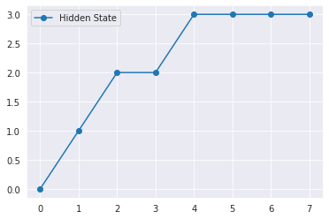
Speech Recognition

Other Applications of Hidden Markov Model

HMMs are widely used in a variety of applications such as speech recognition, natural language processing, computational biology, and finance. In speech recognition, for example, an HMM can be used to model the underlying sounds or phonemes that generate the speech signal, and the observations could be the features extracted from the speech signal. In computational biology, an HMM can be used to model the evolution of a protein or DNA sequence, and the observations could be the sequence of amino acids or nucleotides.

Summary

In summary, HMMs are a powerful tool for modeling sequential data, and their implementation through libraries such as hmmlearn makes them accessible and useful for a variety of applications.

Frequently Asked Questions(FAQs)

Q. 1 What is a Hidden Markov Model (HMM)?

A statistical model called a hidden markov model is used to describe systems that change between states with specific probabilities. The reason it is called “hidden” is that although the states produce observable outputs or emissions, they are not directly observable.

Q. 2 What are the key components of an HMM?

States, emission probabilities connected to each state, transition probabilities between states, and an initial probability distribution over states make up an HMM.

Q. 3 How is an HMM different from a regular Markov Model?

Every state in a standard Markov model can be observed directly. On the other hand, only the emissions-the observable outputs-are visible in an HMM, while the states remain hidden.

Q. 4 What are the applications of Hidden Markov Models?

Speech recognition, natural language processing, bioinformatics (gene prediction, for example), and many other fields where systems can be modeled as sequences of observable events with underlying hidden states are applications that heavily rely on HMMs.