Hermite Curve in Computer Graphics

Last Updated : 15 Jul, 2023

In computer graphics, we often need to draw different types of objects onto the screen. Objects are not flat all time and we need to draw curves many times to draw an object.

Before going into Hermite curves, we will discuss in this article about curves. Spline curves are of two types:

1. Approximation Spline Curve: Here the curve passes close to the control point. As we can see in the diagram below. Examples are the Bezier curve, the B-spline curve, etc.

2. Interpolation Spline Curve: In this case, the curve passes through all the control points. An example is the Hermite curve.

Hermite Curve

Hermite curve named after the French mathematician Charles Hermite is an interpolating piecewise cubic polynomial. It has a specified tangent at each control point. Hermite spline curves can be adjusted locally because each section is only dependent on its endpoint constraints.

If $P(k)$ represents a parametric cubic point function for the curve section between control points P_kand P, then boundary conditions that define the Hermite curve section are

$P(0)= Pk$

$P(1)= P_k+1$

$P'(0)= DPk (derivative of P(0))$

$P'(1)= DP_k+1 (derivative of P(1))$

with DP_k and DP_k+1 specifying the value for parametric derivatives(slope of the curve) at control points P_k and P_k+1. The resulting Hermite curve is something like the below:

As we know Hermite curve is a cubic polynomial. So we will write here:

$P(u)= au^3 +bu^2 +cu+d, where 0<=u<=1$

$Px(u)= axu^3+ bxu^2+ cxu+ dx$

$Py(u)= ayu^3+ byu^2+ cyu+ dy$

$Pz(u)= azu^3+ bzu^2+ cz^u+ dz$

Now we will differentiate the cubic polynomial P(u). On differentiating, we get,

$P'(u)= 3au^2+ 2bu+ c$

Now we will apply the boundary conditions u=0 and u=1 to P(u).

We first apply u=0

$Pk=P(0)= a*0+ b*0+ c*0+ d*1 ----(1)$

The second boundary condition u=1,

$Pk=P(1)= a*1+ b*1+ c*1+ d*1 ------(2)$

For the derivative of P, we apply boundary conditions now. First, we apply u=0

$P'(0)= 3a*0+ 2b*0+ c*1+ d*0 ------(3)$

Now for u=1

$P'(1)= 3a*1+ 2b*1+ c*1+ d*1 ------(4)$

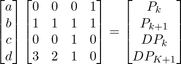
So these are the four linear equations that we get on applying the boundary conditions to P(u) and P'(u). Now we will write these four equations in the form of a matrix as shown in the image below.

$\begin{bmatrix} P(0)\\ P(1)\\ P'(0)\\ P'(1)\\ \end{bmatrix} or \begin{bmatrix} P_{k}\\ P_{k+1}\\ DP_{k}\\ DP_{K+1}\\ \end{bmatrix} = \begin{bmatrix} 0 & 0& 0 & 1\\ 1 & 1& 1 & 1\\ 0& 0 & 1& 0\\ 3& 2& 1 & 0 \end{bmatrix} \begin{bmatrix} a\\ b\\ c\\ d\\ \end{bmatrix}$

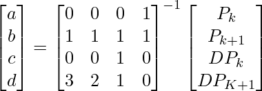
We can calculate the value of a, b, c, and d by performing the required matrix operations as shown below.

$\begin{bmatrix} a\\ b\\ c\\ d\\ \end{bmatrix}\begin{bmatrix} 0 & 0& 0 & 1\\ 1 & 1& 1 & 1\\ 0& 0 & 1& 0\\ 3& 2& 1 & 0 \end{bmatrix} = \begin{bmatrix} P_{k}\\ P_{k+1}\\ DP_{k}\\ DP_{K+1}\\ \end{bmatrix}$

$\begin{bmatrix} a\\ b\\ c\\ d\\ \end {bmatrix} = \begin{bmatrix} 0 & 0& 0 & 1\\ 1 & 1& 1 & 1\\ 0& 0 & 1& 0\\ 3& 2& 1 & 0 \end{bmatrix}^{-1} \begin{bmatrix} P_{k}\\ P_{k+1}\\ DP_{k}\\ DP_{K+1}\\ \end{bmatrix}$

$\begin{bmatrix} a\\ b\\ c\\ d\\ \end {bmatrix} = \begin{bmatrix} 2 & -2& 1& 1\\ -3 & 3 & -2 & -1\\ 0& 0 & 1 & 0\\ 1& 0 & 0 & 0 \end{bmatrix} \begin{bmatrix} P_{k}\\ P_{k+1}\\ DP_{k}\\ DP_{K+1}\\ \end{bmatrix}$

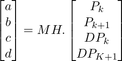
The matrix calculated above is known as the Hermite matrix and is denoted by M_H. So we can write the equation as shown below.

$\begin{bmatrix} a\\ b\\ c\\ d\\ \end {bmatrix} = MH . \begin{bmatrix} P_{k}\\ P_{k+1}\\ DP_{k}\\ DP_{K+1}\\ \end{bmatrix}$

we know that $P(u)= au^{3}+bu^3+cu+d$

$P(u)= u^{3}+u^2+u+1 \begin{bmatrix} a\\ b\\ c\\ d\\ \end {bmatrix} = u+u+u+1 . MH \begin{bmatrix} P_{k}\\ P_{k+1}\\ DP_{k}\\ DP_{K+1}\\ \end{bmatrix}$

After multiplying the matrices on the right-hand side in the above image, we will get:

$P(u)= Pk (2u3 - 3u2 + 1) + Pk+1(-2u3+3u2) + DPk(u3-2u2+u) + DPk+1(u3-u2)$

$P(u)= PkH0(u) + Pk+1H1(u) + DPkH2(u) + DPk+1H3(u)$

where H₀, H₁, H₂, H₃are Hermite blending function.

Hermite Blending Functions

Conceptual Realignment
Curves are weighted averages of points/vectors.
Blending functions specify the weighting.

Application

The Hermite curve is used to interpolate sample points on a 2-D plane that results in a smooth curve, but not a free form, unlike the Bezier and B-spline curves. The most commonly used cubic spline is a 3-D planar curve.

Advantages

Hermite curves are easily calculatable. They are used to smoothly interpolate through control points. Understanding the mathematical background of Hermite curves will help us to understand the entire family of splines.

Disadvantages

First-order derivatives are required; it is not suitable for a designer to provide first-order derivatives.
There is no local control support.
The order of the curve is constant in spite of the number of data points.
Physically, the values of parameters that is the blending function H0, H1, H2, and H3 do not contain any meaning. If we know these values, we can’t imagine the shape of the curve.

Suggest improvement

Computer Graphics Curve in Computer Graphics

Share your thoughts in the comments

Hermite Curve in Computer Graphics

Hermite Curve

Hermite Blending Functions

Application

Advantages

Disadvantages

Please Login to comment...

Similar Reads

What kind of Experience do you want to share?