Open Addressing:
Like separate chaining, open addressing is a method for handling collisions. In Open Addressing, all elements are stored in the hash table itself. So at any point, the size of the table must be greater than or equal to the total number of keys (Note that we can increase table size by copying old data if needed). This approach is also known as closed hashing. This entire procedure is based upon probing. We will understand the types of probing ahead:
- Insert(k): Keep probing until an empty slot is found. Once an empty slot is found, insert k.
- Search(k): Keep probing until the slot’s key doesn’t become equal to k or an empty slot is reached.
- Delete(k): Delete operation is interesting. If we simply delete a key, then the search may fail. So slots of deleted keys are marked specially as “deleted”.
The insert can insert an item in a deleted slot, but the search doesn’t stop at a deleted slot.
Different ways of Open Addressing:
1. Linear Probing:
In linear probing, the hash table is searched sequentially that starts from the original location of the hash. If in case the location that we get is already occupied, then we check for the next location.
The function used for rehashing is as follows: rehash(key) = (n+1)%table-size.
For example, The typical gap between two probes is 1 as seen in the example below:
Let hash(x) be the slot index computed using a hash function and S be the table size
If slot hash(x) % S is full, then we try (hash(x) + 1) % S
If (hash(x) + 1) % S is also full, then we try (hash(x) + 2) % S
If (hash(x) + 2) % S is also full, then we try (hash(x) + 3) % S
…………………………………………..
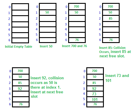
…………………………………………..Let us consider a simple hash function as “key mod 7” and a sequence of keys as 50, 700, 76, 85, 92, 73, 101,
which means hash(key)= key% S, here S=size of the table =7,indexed from 0 to 6.We can define the hash function as per our choice if we want to create a hash table,although it is fixed internally with a pre-defined formula.
Applications of linear probing:
Linear probing is a collision handling technique used in hashing, where the algorithm looks for the next available slot in the hash table to store the collided key. Some of the applications of linear probing include:
- Symbol tables: Linear probing is commonly used in symbol tables, which are used in compilers and interpreters to store variables and their associated values. Since symbol tables can grow dynamically, linear probing can be used to handle collisions and ensure that variables are stored efficiently.
- Caching: Linear probing can be used in caching systems to store frequently accessed data in memory. When a cache miss occurs, the data can be loaded into the cache using linear probing, and when a collision occurs, the next available slot in the cache can be used to store the data.
- Databases: Linear probing can be used in databases to store records and their associated keys. When a collision occurs, linear probing can be used to find the next available slot to store the record.
- Compiler design: Linear probing can be used in compiler design to implement symbol tables, error recovery mechanisms, and syntax analysis.
- Spell checking: Linear probing can be used in spell-checking software to store the dictionary of words and their associated frequency counts. When a collision occurs, linear probing can be used to store the word in the next available slot.
Overall, linear probing is a simple and efficient method for handling collisions in hash tables, and it can be used in a variety of applications that require efficient storage and retrieval of data.
Challenges in Linear Probing :
- Primary Clustering: One of the problems with linear probing is Primary clustering, many consecutive elements form groups and it starts taking time to find a free slot or to search for an element.
- Secondary Clustering: Secondary clustering is less severe, two records only have the same collision chain (Probe Sequence) if their initial position is the same.
Example: Let us consider a simple hash function as “key mod 5” and a sequence of keys that are to be inserted are 50, 70, 76, 93.
- Step1: First draw the empty hash table which will have a possible range of hash values from 0 to 4 according to the hash function provided.
Hash table
- Step 2: Now insert all the keys in the hash table one by one. The first key is 50. It will map to slot number 0 because 50%5=0. So insert it into slot number 0.
Insert 50 into hash table
- Step 3: The next key is 70. It will map to slot number 0 because 70%5=0 but 50 is already at slot number 0 so, search for the next empty slot and insert it.
Insert 70 into hash table
- Step 4: The next key is 76. It will map to slot number 1 because 76%5=1 but 70 is already at slot number 1 so, search for the next empty slot and insert it.
Insert 76 into hash table
- Step 5: The next key is 93 It will map to slot number 3 because 93%5=3, So insert it into slot number 3.
Insert 93 into hash table
2. Quadratic Probing
If you observe carefully, then you will understand that the interval between probes will increase proportionally to the hash value. Quadratic probing is a method with the help of which we can solve the problem of clustering that was discussed above. This method is also known as the mid-square method. In this method, we look for the i2‘th slot in the ith iteration. We always start from the original hash location. If only the location is occupied then we check the other slots.
let hash(x) be the slot index computed using hash function.
If slot hash(x) % S is full, then we try (hash(x) + 1*1) % S
If (hash(x) + 1*1) % S is also full, then we try (hash(x) + 2*2) % S
If (hash(x) + 2*2) % S is also full, then we try (hash(x) + 3*3) % S
…………………………………………..
…………………………………………..
Example: Let us consider table Size = 7, hash function as Hash(x) = x % 7 and collision resolution strategy to be f(i) = i2 . Insert = 22, 30, and 50.
- Step 1: Create a table of size 7.
Hash table
-
Step 2 – Insert 22 and 30
- Hash(22) = 22 % 7 = 1, Since the cell at index 1 is empty, we can easily insert 22 at slot 1.
- Hash(30) = 30 % 7 = 2, Since the cell at index 2 is empty, we can easily insert 30 at slot 2.
Insert keys 22 and 30 in the hash table
-
Step 3: Inserting 50
- Hash(50) = 50 % 7 = 1
- In our hash table slot 1 is already occupied. So, we will search for slot 1+12, i.e. 1+1 = 2,
- Again slot 2 is found occupied, so we will search for cell 1+22, i.e.1+4 = 5,
- Now, cell 5 is not occupied so we will place 50 in slot 5.
Insert key 50 in the hash table
3. Double Hashing
The intervals that lie between probes are computed by another hash function. Double hashing is a technique that reduces clustering in an optimized way. In this technique, the increments for the probing sequence are computed by using another hash function. We use another hash function hash2(x) and look for the i*hash2(x) slot in the ith rotation.
let hash(x) be the slot index computed using hash function.
If slot hash(x) % S is full, then we try (hash(x) + 1*hash2(x)) % S
If (hash(x) + 1*hash2(x)) % S is also full, then we try (hash(x) + 2*hash2(x)) % S
If (hash(x) + 2*hash2(x)) % S is also full, then we try (hash(x) + 3*hash2(x)) % S
…………………………………………..
…………………………………………..
Example: Insert the keys 27, 43, 692, 72 into the Hash Table of size 7. where first hash-function is h1(k) = k mod 7 and second hash-function is h2(k) = 1 + (k mod 5)
-
Step 1: Insert 27
- 27 % 7 = 6, location 6 is empty so insert 27 into 6 slot.
Insert key 27 in the hash table
-
Step 2: Insert 43
- 43 % 7 = 1, location 1 is empty so insert 43 into 1 slot.
Insert key 43 in the hash table
-
Step 3: Insert 692
- 692 % 7 = 6, but location 6 is already being occupied and this is a collision
- So we need to resolve this collision using double hashing.
hnew = [h1(692) + i * (h2(692)] % 7
= [6 + 1 * (1 + 692 % 5)] % 7
= 9% 7
= 2Now, as 2 is an empty slot,
so we can insert 692 into 2nd slot.
Insert key 692 in the hash table
-
Step 4: Insert 72
- 72 % 7 = 2, but location 2 is already being occupied and this is a collision.
- So we need to resolve this collision using double hashing.
hnew = [h1(72) + i * (h2(72)] % 7
= [2 + 1 * (1 + 72 % 5)] % 7
= 5 % 7
= 5,Now, as 5 is an empty slot,
so we can insert 72 into 5th slot.
Insert key 72 in the hash table
See this for step-by-step diagrams:
Comparison of the above three:
Open addressing is a collision handling technique used in hashing where, when a collision occurs (i.e., when two or more keys map to the same slot), the algorithm looks for another empty slot in the hash table to store the collided key.
- In linear probing, the algorithm simply looks for the next available slot in the hash table and places the collided key there. If that slot is also occupied, the algorithm continues searching for the next available slot until an empty slot is found. This process is repeated until all collided keys have been stored. Linear probing has the best cache performance but suffers from clustering. One more advantage of Linear probing is easy to compute.
- In quadratic probing, the algorithm searches for slots in a more spaced-out manner. When a collision occurs, the algorithm looks for the next slot using an equation that involves the original hash value and a quadratic function. If that slot is also occupied, the algorithm increments the value of the quadratic function and tries again. This process is repeated until an empty slot is found. Quadratic probing lies between the two in terms of cache performance and clustering.
- In double hashing, the algorithm uses a second hash function to determine the next slot to check when a collision occurs. The algorithm calculates a hash value using the original hash function, then uses the second hash function to calculate an offset. The algorithm then checks the slot that is the sum of the original hash value and the offset. If that slot is occupied, the algorithm increments the offset and tries again. This process is repeated until an empty slot is found. Double hashing has poor cache performance but no clustering. Double hashing requires more computation time as two hash functions need to be computed.
The choice of collision handling technique can have a significant impact on the performance of a hash table. Linear probing is simple and fast, but it can lead to clustering (i.e., a situation where keys are stored in long contiguous runs) and can degrade performance. Quadratic probing is more spaced out, but it can also lead to clustering and can result in a situation where some slots are never checked. Double hashing is more complex, but it can lead to more even distribution of keys and can provide better performance in some cases.
| S.No. | Separate Chaining | Open Addressing |
|---|---|---|
| 1. | Chaining is Simpler to implement. | Open Addressing requires more computation. |
| 2. | In chaining, Hash table never fills up, we can always add more elements to chain. | In open addressing, table may become full. |
| 3. | Chaining is Less sensitive to the hash function or load factors. | Open addressing requires extra care to avoid clustering and load factor. |
| 4. | Chaining is mostly used when it is unknown how many and how frequently keys may be inserted or deleted. | Open addressing is used when the frequency and number of keys is known. |
| 5. | Cache performance of chaining is not good as keys are stored using linked list. | Open addressing provides better cache performance as everything is stored in the same table. |
| 6. | Wastage of Space (Some Parts of hash table in chaining are never used). | In Open addressing, a slot can be used even if an input doesn’t map to it. |
| 7. | Chaining uses extra space for links. | No links in Open addressing |
Note: Cache performance of chaining is not good because when we traverse a Linked List, we are basically jumping from one node to another, all across the computer’s memory. For this reason, the CPU cannot cache the nodes which aren’t visited yet, this doesn’t help us. But with Open Addressing, data isn’t spread, so if the CPU detects that a segment of memory is constantly being accessed, it gets cached for quick access.
Performance of Open Addressing:
Like Chaining, the performance of hashing can be evaluated under the assumption that each key is equally likely to be hashed to any slot of the table (simple uniform hashing)
m = Number of slots in the hash table
n = Number of keys to be inserted in the hash table
Load factor α = n/m ( < 1 )
Expected time to search/insert/delete < 1/(1 – α)
So Search, Insert and Delete take (1/(1 – α)) time
Related Articles: Hashing | Set 1 (Introduction), Hashing | Set 2 (Separate Chaining)