Grey wolf optimization – Introduction

Optimization is essentially everywhere, from engineering design to economics and from holiday planning to Internet routing. As money, resources and time are always limited, the optimal utilization of these available resources is crucially important.

In general, an optimization problem can be written as  

optimize  , 
subject to,  
                      , 
                      , (

where f₁, …, f_N are the objectives, while h_j and g_k are the equality and inequality constraints, respectively. In the case when N=1, it is called single-objective optimization. When N≥2, it becomes a multi-objective optimization problem whose solution strategy is different from those for a single objective. This article mainly concerns single-objective optimization problems.

Different types of optimization algorithms

Deterministic optimization algorithms:  

Deterministic approaches take advantage of the analytical properties of the problem to generate a sequence of points that converge to a globally optimal solution. These approaches can provide general tools for solving optimization problems to obtain a global or approximately global optimum.

Examples: linear programming, nonlinear programming, and mixed-integer nonlinear programming, etc.

Heuristics and metaheuristics:

A meta heuristic is a higher-level procedure or heuristic which aims to find, generate, or select a heuristic (partial search algorithm) that may provide a sufficiently good solution to an optimization problem. They are used especially when incomplete or imperfect information is available or when there is limited computation capacity.

Meta heuristics make relatively few assumptions about the optimization problem being solved and so may be usable for a variety of problems.  

Examples: Particle Swarm Optimization (PSO), Ant Colony Optimization (ACO), Genetic Algorithms (GA), Cuckoo search algorithm, Grey wolf optimization (GWO) etc.

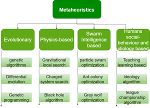
Figure 1: Classification of metaheuristic algorithms with examples from each class

This article aims to introduce the basics of a novel metaheuristic called Grey wolf optimization (GWO)

Inspiration of the algorithm

Grey wolf optimizer (GWO) is a population-based meta-heuristics algorithm that simulates the leadership hierarchy and hunting mechanism of grey wolves in nature, and it’s proposed by Seyedali Mirjalili et al. in 2014.  

• Grey wolves are considered apex predators, which are at the top of the food chain
• Grey wolves prefer to live in groups (packs), each group contain 5-12 individuals on average.
• All the individuals in the group have a very strict social dominance hierarchy as demonstrated in the accompanying figure.

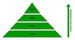
Figure 2: Social hierarchy of Grey wolves

1. Alpha α wolf is considered the dominant wolf in the pack and his/her orders should be followed by the pack members.
2. Beta β are subordinate wolves, which help the alpha in decision-making and are considered as the best candidate to be the alpha.
3. Delta δ wolves have to submit to the alpha and beta, but they dominate the omega. There are different categories of delta-like Scouts, Sentinels, Elders, Hunters, Caretakers etc.
4. Omega ω wolves are considered as the scapegoat in the pack, are the least important individuals in the pack and are only allowed to eat at last.

Main phases of grey wolf hunting:

1. Tracking, chasing and approaching the prey.
2. Pursuing, encircling, and harassing the prey until it stops moving.
3. Attack towards the prey.

The social hierarchy and hunting behaviour of grey wolves are mathematically modeled to design GWO.

Mathematical model and algorithm: 

Social hierarchy: 

• The Fittest solution as an Alpha wolf (α)
• Second best solution as a Beta wolf (β)
• Third best solution as a Delta wolf (δ)
• Rest of the candidate solutions as Omega wolves (ω)

Encircling the Prey: 

                             (1)

                              (2)

Where t indicates the current iteration, and  are coefficient vectors,  is the position vector of the prey, and indicates the position vector of a grey wolf.

    and                      (3)

components of  are linearly decreased from 2 to 0 over the course of iterations and ,  are random vectors in [0, 1].

Hunting: 

In each iteration, omega wolves update their positions in accordance with the positions α, β, and δ alpha, beta, and delta because α, β, and δ have better knowledge about the potential location of prey.

  ,   ,                              (4)

  ,    ,                     (5)

                 (6)

Attacking prey (exploitation): 

When prey stops moving then grey wolf finish the hunting by attacking the prey and to mathematically model that we decrease the value of .  is a random value in the interval [-2a, 2a], where a is decreased from 2 to 0 over course of iterations.  

|A|<1 force the wolves to attack the prey ( exploitation)

Searching for prey ( exploration): 

|A|>1 forces the grey wolves to diverge from the prey to hopefully find a fitter prey ( exploitation)

Another component of GWO that favours exploration is . It contains random value between [0, 2]. C>1 emphasize the attack while C<1 deemphasize the attack.

Pseudocode of the GWO algorithm: 

• Step1: Randomly initialize the population of grey wolves X_i (i=1,2,…,n)
• Step2: Initialize the value of a=2, A and C  ( using eq.3)
• Step3: Calculate the fitness of each member of the population
  • X_α=member with the best fitness value
  • X_β=second best member ( in terms of fitness value)
  • X_δ=third best member (in terms of fitness value)
• Step4: FOR t = 1 to Max_number_of_iterations:
  • Update the position of all the omega wolves by eq. 4, 5 and 6
  • Update a, A, C (using eq. 3)
  • a = 2(1-t/T)
  • Calculate Fitness of all search agents
  • Update Xα, Xβ, Xδ.
  •             END FOR
• Step5: return X_α

References: 

• https://www.sciencedirect.com/science/article/pii/S0965997813001853
• https://www.slideshare.net/afar1111/grey-wolf-optimizer