Graphs, Automatic Differentiation and Autograd in PyTorch

Graphs, Automatic Differentiation and Autograd are powerful tools in PyTorch that can be used to train deep learning models. Graphs are used to represent the computation of a model, while Automatic Differentiation and Autograd allow the model to learn by updating its parameters during training. In this article, we will explore the concepts behind these tools and how they can be used in PyTorch.

Graphs: A graph is a data structure that is used to represent the computation of a model. In PyTorch, a graph is represented by a directed acyclic graph (DAG), where each node represents a computation, and the edges represent the flow of data between computations. The graph is used to track the dependencies between computations and to compute gradients during the backpropagation step.

Automatic Differentiation: Automatic Differentiation (AD) is a technique that allows the model to compute gradients automatically. In PyTorch, AD is implemented through the Autograd library, which uses the graph structure to compute gradients. AD allows the model to learn by updating its parameters during training, without the need for manual computation of gradients.

Autograd: Autograd is a PyTorch library that implements Automatic Differentiation. It uses the graph structure to compute gradients and allows the model to learn by updating its parameters during training. Autograd also provides a way to compute gradients with respect to arbitrary scalar values, which is useful for tasks such as optimization.

Using Graphs, Automatic Differentiation, and Autograd in PyTorch

The steps involved in using Graphs, Automatic Differentiation, and Autograd in PyTorch are as follows:

1. Define the graph structure: The first step in using these concepts in PyTorch is to define the graph structure of the model. This can be done by creating tensors and operations on them.
2. Enable Autograd: Once the graph structure is defined, Autograd needs to be enabled on the tensors that require gradients. This can be done by setting the “requires_grad” attribute to True.
3. Forward pass: After the graph structure is defined and Autograd is enabled, the forward pass can be performed. This involves computing the output of the model given an input.
4. Backward pass: Once the forward pass is complete, the backward pass can be performed to compute the gradients. This is done by calling the “backward()” method on the output tensor.
5. Update parameters: Finally, the gradients can be used to update the parameters of the model using an optimizer.

To plot the computational graph graphviz and torchviz should be installed in the system

sudo apt install graphviz   # [Ubuntu]
winget install graphviz     # [Windows]
sudo port install graphviz  # [Mac]

pip install torchviz

Examples 1:

1.  Import the torch library
2.  Create a tensor input value with requires_grad = True. Basically, this is used to record the autograd operations.
3.  Define the function.
4.  Use f.backward() to execute the backward pass and computes all the backpropagation gradients automatically.
5. Calculate the derivative value of the given function for the given input using x.grad
6. Plot the computational graph using the torchviz make_dot() function.
7. Note  Here the input should be float value.

Python3

# Import the torch library
import torch
from torchviz import make_dot

# Assign any value for x as tensor form
# Set requires_grad=True So,
# that autograd will record the operations
x=torch.tensor(7.0,requires_grad=True)

# Define the equation
f = (x**2)+3

# Differentiate using torch
#Uses backward function to compute the gradient value
f.backward()

# Print the derivative value
# of y i.e dy/dx = 2x  = 2 X 7.0 = 14.
print(x.grad)

# Plot the computational graph
make_dot(f)

Output:

tensor(14.)

computational graph

Examples 2:

1.  Import the torch library
2.  Create a tensor input value with requires_grad = True. Basically, this is used to record the autograd operations.
3.  Define the function.
4. Create a variable z with the sum of f(x). Because torch.autograd.grad() works only for scalar input. 
5.  Use z.backward() to execute the backward pass and computes all the backpropagation gradients automatically.
6. Calculate the derivative value of the given function for the given input using x.grad
7. Plot the computational graph using the torchviz make_dot() function.

Note: Here the input should be float value.

Python3

# import the library
import torch
from torchviz import make_dot

# Assign the input variable
x = torch_input=torch.tensor([[1.0,2.0,3.0],
                              [4.0,5.0,6.0],
                              [7.0,8.0,9.0]],requires_grad=True)

# define the function
def f(x):
    return (x**3) + 7*(x**2) + 5*x + 10

# Assign the sum to another variable z
z=f(x).sum()

# Compute the gradient
z.backward()

# Find the gradient value
print(x.grad)

#Plot the computational graph
make_dot(z)

Output:

tensor([[ 22.,  45.,  74.],
        [109., 150., 197.],
        [250., 309., 374.]])

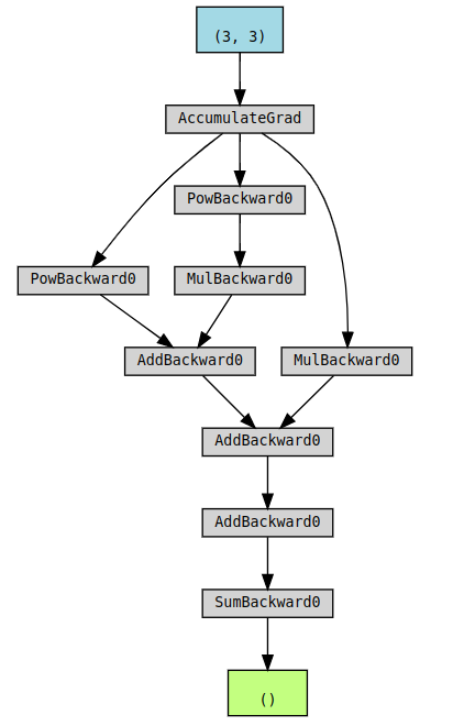
computational graph

Example 3: A simple linear regression model

Python3

# Import the torch library
import torch
from torchviz import make_dot

# Define Input variable
x = torch.randn(1, requires_grad=True)
w = torch.randn(1, requires_grad=True)
b = torch.randn(1, requires_grad=True)

# Define the graph structure
# Forward pass
y = w * x + b

# Backward pass
y.backward()

#View the outputs
print("Gradient of x:", x.grad)
print("Gradient of b:", b.grad)
print("Gradient of w:", w.grad)

# Update parameters
w.data -= 0.01 * w.grad.data
b.data -= 0.01 * b.grad.data

# Plot the computational graph
make_dot(y)

Output:

Gradient of x: tensor([0.9148])
Gradient of b: tensor([1.])
Gradient of w: tensor([1.3919])

computational graph

Example 4: A Simple Neural Network with a Single Hidden Layer

Python3

# Import the torch library
import torch
from torchviz import make_dot

# Input
x = torch.randn(1, 10, requires_grad=True)
w1 = torch.randn(10, 5, requires_grad=True)
b1 = torch.randn(5, requires_grad=True)

# Forward pass
h = x @ w1 + b1
h = torch.relu(h)

w2 = torch.randn(5, 1, requires_grad=True)
b2 = torch.randn(1, requires_grad=True)
y = h @ w2 + b2

# Backward pass
y.backward()

#view the outputs
print("Gradient of w1:", w1.grad)
print("Gradient of b1:", b1.grad)
print("Gradient of w2:", w2.grad)
print("Gradient of b2:", b2.grad)

# Update parameters
w1.data -= 0.01 * w1.grad.data
b1.data -= 0.01 * b1.grad.data
w2.data -= 0.01 * w2.grad.data
b2.data -= 0.01 * b2.grad.data

# Plot the computational graph
make_dot(y)

Output:

Gradient of w1: tensor([[-0.0000, -0.0000,  0.0090, -0.0000, -0.2808],
        [-0.0000, -0.0000,  0.0638, -0.0000, -1.9863],
        [-0.0000, -0.0000,  0.0094, -0.0000, -0.2912],
        [-0.0000, -0.0000,  0.0049, -0.0000, -0.1519],
        [-0.0000, -0.0000,  0.0871, -0.0000, -2.7127],
        [-0.0000, -0.0000,  0.0614, -0.0000, -1.9097],
        [-0.0000, -0.0000,  0.0031, -0.0000, -0.0957],
        [ 0.0000,  0.0000, -0.0503,  0.0000,  1.5671],
        [-0.0000, -0.0000,  0.0080, -0.0000, -0.2488],
        [-0.0000, -0.0000,  0.0974, -0.0000, -3.0309]])
Gradient of b1: tensor([ 0.0000,  0.0000, -0.0503,  0.0000,  1.5665])
Gradient of w2: tensor([[0.0000],
        [0.0000],
        [3.9794],
        [0.0000],
        [0.6139]])
Gradient of b2: tensor([1.])

computational graph 

Note: The output for the examples may be different because of the use of random initializations for the weights and biases. The values are randomly generated at each run, leading to different outputs. In general, it’s a common practice in deep learning to initialize the weights randomly, as this helps to break the symmetry and encourages the network to learn a diverse set of solutions. The gradients of these variables will also change during the backward pass based on the random initialization, so the outputs will be different each time you run the code.

Conclusion:

In conclusion, Graphs, Automatic Differentiation, and Autograd are powerful tools in PyTorch for building and training machine learning models. In Example 1, we showed how to define the computation graph, perform a forward pass to calculate the output, and perform a backward pass to calculate the gradients. In Example 2, we demonstrate how these concepts can be applied to building and training a simple neural network with a single hidden layer. These examples serve as a starting point for further exploration and experimentation. Whether you are a seasoned machine learning practitioner or a beginner, understanding the concepts and capabilities of Graphs, Automatic Differentiation, and Autograd is essential for building and training effective machine learning models in PyTorch.