Graph Matrices in Software Testing

A graph matrix is a data structure that can assist in developing a tool for automation of path testing. Properties of graph matrices are fundamental for developing a test tool and hence graph matrices are very useful in understanding software testing concepts and theory.

What is a Graph Matrix ?
A graph matrix is a square matrix whose size represents the number of nodes in the control flow graph. If you do not know what control flow graphs are, then read this article. Each row and column in the matrix identifies a node and the entries in the matrix represent the edges or links between these nodes. Conventionally, nodes are denoted by digits and edges are denoted by letters.

Let’s take an example.

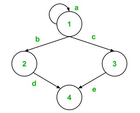
Let’s convert this control flow graph into a graph matrix. Since the graph has 4 nodes, so the graph matrix would have a dimension of 4 X 4. Matrix entries will be filled as follows :

• (1, 1) will be filled with ‘a’ as an edge exists from node 1 to node 1
• (1, 2) will be filled with ‘b’ as an edge exists from node 1 to node 2. It is important to note that (2, 1) will not be filled as the edge is unidirectional and not bidirectional
• (1, 3) will be filled with ‘c’ as edge c exists from node 1 to node 3
• (2, 4) will be filled with ‘d’ as edge exists from node 2 to node 4
• (3, 4) will be filled with ‘e’ as an edge exists from node 3 to node 4

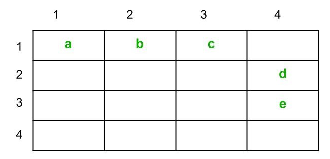
The graph matrix formed is shown below :

Connection Matrix :
A connection matrix is a matrix defined with edges weight. In simple form, when a connection exists between two nodes of control flow graph, then the edge weight is 1, otherwise, it is 0. However, 0 is not usually entered in the matrix cells to reduce the complexity.

For example, if we represent the above control flow graph as a connection matrix, then the result would be :

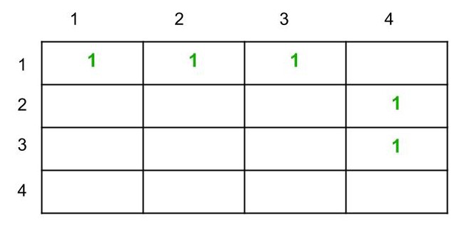
As we can see, the weight of the edges are simply replaced by 1 and the cells which were empty before are left as it is, i.e., representing 0.

A connection matrix is used to find the cyclomatic complexity of the control graph.
Although there are three other methods to find the cyclomatic complexity but this method works well too.

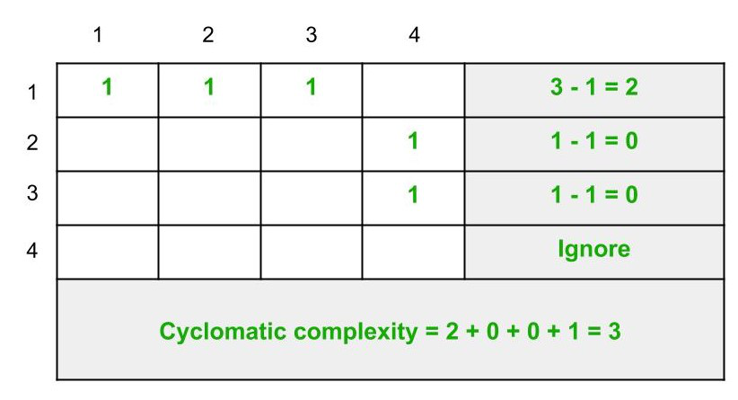
Following are the steps to compute the cyclomatic complexity :

1. Count the number of 1s in each row and write it in the end of the row
2. Subtract 1 from this count for each row (Ignore the row if its count is 0)
3. Add the count of each row calculated previously
4. Add 1 to this total count
5. The final sum in Step 4 is the cyclomatic complexity of the control flow graph

Let’s apply these steps to the graph above to compute the cyclomatic complexity.

We can verify this value for cyclomatic complexity using other methods :

Method-1 :

Cyclomatic complexity
= e - n + 2 * P 

Since here,

e = 5
n = 4
and, P = 1 

Therefore, cyclomatic complexity,

= 5 - 4 + 2 * 1 
= 3 

Method-2 :

Cyclomatic complexity 
= d + P 

Here,

d = 2 
and, P = 1 

Therefore, cyclomatic complexity,

= 2 + 1 
= 3 

Method-3:

Cyclomatic complexity
= number of regions in the graph 

li

• Region 1: bounded by edges b, c, d, and e
• Region 2: bounded by edge a (in loop)
• Region 3: outside the graph

Therefore, cyclomatic complexity,

= 1 + 1 + 1 
= 3 

It can be seen that all other methods give the same result. Method1, 2, and 3 have been discussed here in detail.