How to use Goal Seek in Excel for What-If analysis with Examples

Goal Seek is a “What if – analysis” tool available in MS EXCEL to determine or calculate any input value based on the formula and the output/resultant value. In simple language, we can say, “What should be the input value of the given output”? The good thing about Goal Seek is that it performs all calculations behind the scenes. You are only asked to give these three parameters Set cell, To value, By changing cell.

What is Goal Seek in Excel

The Goal Seek in Excel is a built-in What-if-Analysis tool that helps us to know how one value in a formula impacts another. It also determines what should be given as input to attain the desired output. The Goal Seek tool is especially useful for doing sensitivity analysis. It has many uses.

Where to Find Goal Seek in Excel

Step 1: Go to the Data Tab in MS Excel

Step 2: In the Data Tools group, you will find a What-if analysis

Step 3: Click on What if analysis, and you will find Goal Seek

Goal seek dialogue box has three parts:

1. Set Cell: In this, we write the reference of the cell which contains the formula.
2. To value: In this, we write the value which we want to attain(or the given resultant value).
3. By changing Cell: In this, we write the reference of the cell whose value we want to change(i.e. the cell whose value is to be calculated).

Note: Goal seek works with only one variable input at given time. You can use the Solver in Excel for multiple input values.

How to Use Goal Seek in Excel – Example 1

Determine the Rate Of Interest using a Simple Interest.  

We need to calculate the rate of interest when the time period, principal amount, and simple interest are already known.

Given

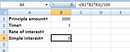
Principle amount = 2000

Time = 3 Years

Simple interest = 6000

Step 1: Open MS Excel and Insert the Values

Step 2: Write the formula of Simple Interest in any one cell (B4)

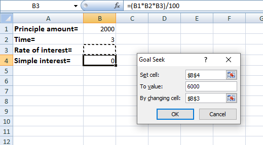
Step 3: Open the Goal Seek Dialogue Box

Step 4: Choose the Simple Interest Formula Cell (B4)

In the Set Cell box select the cell which contains the formula of simple interest (B4)

Step 5: Enter 6000 (as given) in the To Value Box

In the To Value box write the resultant value of the simple interest i.e. 6000 (Given in question).

Step 6: Enter the rate of interest cell reference (B3) in the By Changing Cell

In the By Changing Cell write the reference of the cell in which you want the rate of interest value (B3).

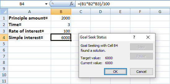
Step 7: Click Ok

Step 8: Preview the Result

The Rate of interest value is calculated in cell (B3).

Things to Remember 

• There should always be a formula in “set cell”, It can’t be empty.
• There should be dependency of “set cell” directly or indirectly on “by changing cell”. That is necessary to study the imapct on the “set cell”.
• The “by changing cell” should not contain any special characters.

Note: The formula remains the same throughout. The input values entered in the “by changing cell” box are changed to study the effect on the output.

How to Use Goal Seek in Excel – Example 2

Determine the Value of the unit if the Sum is given. We have to calculate the value, when the Sum of the values is 303.

Step 1: Enter the values in the Cells

Step 2: Write the Formula of SUM() in any Cell

Step 3: Click Data tab and Go to What-if Analysis and Select Goal Seek

Now click on the Data tab in the Ribbon, and select the option What-if-analysis to open Goal Seek.

Step 4: Select the cell which contains the formula

In the Set cell Box, Select the cell which contains the formula.

Step 5: Write the Resultant value of total, 303 (given)

In the To value box, Write the Resultant value of total, 303 (given).

Step 6: Write the Reference of the cell in Which you Want the Value

In the by-changing cell, Write the reference of the cell in which you want the value. 

Step 7: Click Ok

The output of Unit 5 is given in the above image, Hence the value of Unit 5 is 89 to attain the Value of the total.

How to Goal Seek in Excel – Example 3

What-if-analysis of the Student performance

You have to find the marks of a particular subject of the student if the final average is 83 (given).

Step 1: Enter the marks of different subjects of a student in Excel.

Step 2: Now Go to the Data tab in Ribbon and select Goal Seek from the Drop Down menu.

Step 3: Now Enter the values in the dialog box, In the Set cell Box, Select the cell which contains the formula.

Step 5: In the To value box, Write the Resultant value of Average, 83 (given).

Step 6: In the by-changing cell, Write the reference of the cell in which you want the value.

Step 7: Click ‘ok’.

The marks of the computer are given in the above image, Hence the mark of the Computer is 66 to attain the desired output.

Shortcut for Goal Seek in Excel

You can access Goal Seek in Excel using a keyboard shortcut by pressing Alt + A, followed by W, and then G.

How to Fix Goal Seek in Excel

Sometimes, Goal Seek can face challenges finding a solution, often because one may not exist. In such cases, Excel will provide its best estimate and let you know with a message like “Goal Seeking may not have found a solution.” If you’re confident that a solution should be attainable for your formula, consider these simple troubleshooting steps:

Step 1: Confirm Goal Seek Settings

• Make sure the “Set cell” points to the cell with your formula.
• Check if the formula cell depends on the “changing cell,” either directly or indirectly.

Step 2: Adjust Iteration Settings

• Navigate to the File Tab
• Click on Options
• Select Formulas and Change the below options
• Increase “Maximum Iterations” to explore more potential solutions.
• Decrease “Maximum Change” for greater precision, especially if your formula requires it.

Step 3: No Circular References

• Ensure that your formulas don’t create circular references, as Goal Seek and Excel formulas work best when they’re not interdependent.
• These steps should help resolve issues when using Excel’s Goal Seek tool for What-If analysis.

FAQs

How to Use Goal Seek In Excel for Multiple Cells

In Excel, you can use “Goal Seek” to change one cell to reach a specific result. But if you want to adjust multiple cells to hit various targets together, you need “Solver.” To use it:

Step 1: Enable Solver

Go to “File” > “Options” > “Add-Ins,” choose “Excel Add-ins,” and check “Solver Add-in.”

Step 2: Create a Worksheet

Set up input cells, output cells with target values, and the relevant formulas.

Step 3: Define Your Goal

Specify what you want to optimize, like maximizing, minimizing, or hitting a specific value, usually in a separate cell.

Step 4: Set Constraints

If input cells have limits, define them.

Step 5: Use Solver

Find it in the “Data” tab, click “Solver” in the “Analysis” group to open the parameters dialog.

Step 6: Configure Solver

Set your objective cell, the target value, the input cells to adjust, and any constraints.

Step 7: Click Solve

Click “Solve” in the dialog. Solver will attempt to find values for input cells to meet your goals.

Step 8: Preview the Result

Solver will tell you if it succeeded. Click “OK” if it did, or adjust constraints/goals if needed.

Solver is great for complex tasks but may require trial and error to set up effectively.

What is Goal Seek in Excel?

The Goal Seek in Excel calculates the input value based on the given output. Goal Seek is used when there is need to study the impact of change in one value on the other.

The Goal Seek  works with one output at a given time. The Goal Seek is used in Scenario Analysis, cause and effect situation, break- even model, Sensitivity Analysis and so on. 

How does the Goal Seek work in Excel?

The Goal Seek does backward calculation. It helps you to determine the value required in a particular cell to produce a desired outcome in another cell by adjusting the value in a third cell.

Below are the steps to show how the Goal seek works in excel.

Step 1: Enter the data on which Goal Seek calculation are need to be performed.

Step 2: Select “Goal Seek” from the “What -if- analysis” drop – down in the Data tab.

Step 3: Enter Parameters and click “OK”.

Note: The initial value scan be resorted by pressing the “undo”.

What is the advantage of Goal Seek in Excel?

The Goal Seek allows the user to determine the desired input value for a formula when the output value is already known. 

How to Automate Goal Seek in Excel using VBA?

By writing a VBA Macro, you can programmatically specify the target cell, the input cell to adjust, and the desired result. This allows you to perform Goal Seek calculations automatically. 

What are the limitations of using Goal Seek in Excel?

The following are the limitations of Goal seek :

• Only works with single variable.
• Changing one input directly affects the desired output. So, it is advisable to make the calculation clear and effect relationship.