Gauss’s Forward Interpolation

Interpolation refers to the process of creating new data points given within the given set of data. The below code computes the desired data point within the given range of discrete data sets using the formula given by Gauss and this method is known as Gauss’s Forward Method. 

Gauss’s Forward Method:

The gaussian interpolation comes under the Central Difference Interpolation Formulae. Suppose we are given the following value of y=f(x) for a set values of x:
X: x0 x1 x2 ………. xn 
Y: y0 y1 y2 ………… yn 
The differences y1 – y0, y2 – y1, y3 – y2, ……, yn – yn–1 when denoted by Δy0, Δy1, Δy2, ……, Δyn–1 are respectively, called the first forward differences. Thus the first forward differences are :
Δy₀ = y₁ – y₀
and in the same way we can calculate higher order differences.

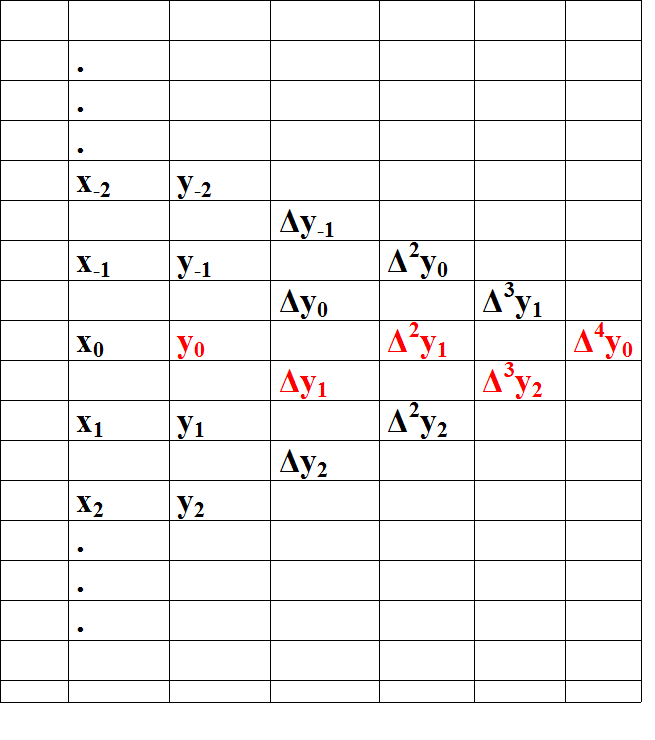
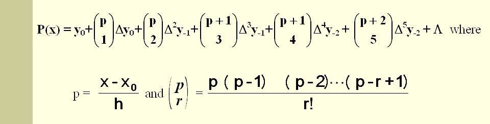
And after the creating table we calculate the value on the basis of following formula:

Now, Let’s take an example and solve it for better understanding. 
Problem: 
From the following table, find the value of e^1.17 using Gauss’s Forward formula.

x	1.00	1.05	1.10	1.15	1.20	1.25	1.30
ex	2.7183	2.8577	3.0042	3.1582	3.3201	3.4903	3.6693

Solution:
We have 
y_p = y₀ + pΔy₀ + (p(p-1)/2!).Δy²₀ + ((p+1)p(p-1)/3!).Δy³₀ + …
where p = (x_1.17 – x_1.15) / h 
and h = x₁ – x₀ = 0.05
so, p = 0.04
Now, we need to calculate Δy₀, Δy²₀, Δy³₀ … etc. 

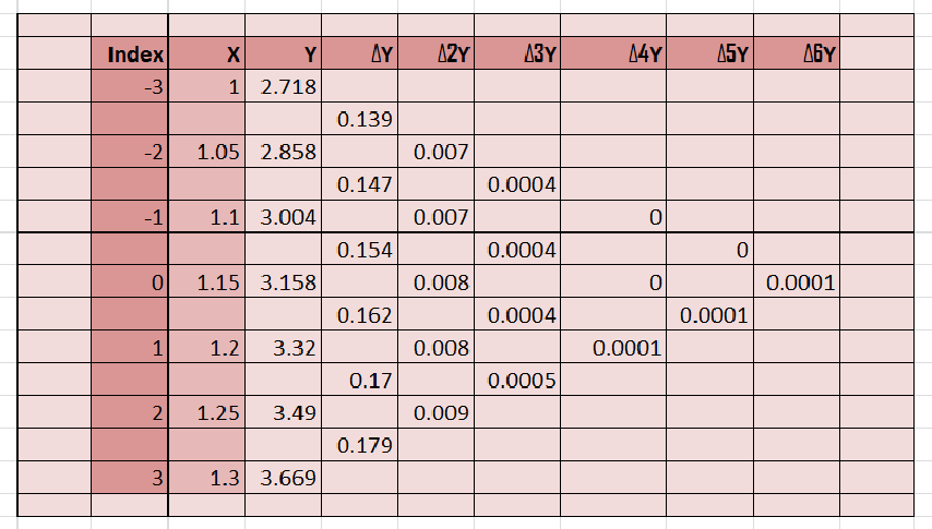
Put the required values in the formula- 
y_{x = 1.17} = 3.158 + (2/5)(0.162) + (2/5)(2/5 – 1)/2.(0.008) … 
y_{x = 1.17} = 3.2246
Code: Python code for implementing Gauss’s Forward Formula

Python3

# Python3 code for Gauss's Forward Formula
# importing library
import numpy as np

# function for calculating coefficient of Y
def p_cal(p, n):

    temp = p;
    for i in range(1, n):
         if(i%2==1):
             temp * (p - i)
         else:
             temp * (p + i)
    return temp;
# function for factorial
def fact(n):
    f = 1
    for i in range(2, n + 1):
        f *= i
    return f

# storing available data
n = 7;
x = [ 1, 1.05, 1.10, 1.15, 1.20, 1.25, 1.30 ];

y = [[0 for i in range(n)]
        for j in range(n)];
y[0][0] = 2.7183;
y[1][0] = 2.8577;
y[2][0] = 3.0042;
y[3][0] = 3.1582;
y[4][0] = 3.3201;
y[5][0] = 3.4903;
y[6][0] = 3.6693;

# Generating Gauss's triangle
for i in range(1, n):
    for j in range(n - i):
        y[j][i] = np.round((y[j + 1][i - 1] - y[j][i - 1]),4);

# Printing the Triangle
for i in range(n):
    print(x[i], end = "\t");
    for j in range(n - i):
        print(y[i][j], end = "\t");
    print("");

# Value of Y need to predict on
value = 1.17;

# implementing Formula
sum = y[int(n/2)][0];
p = (value - x[int(n/2)]) / (x[1] - x[0])

for i in range(1,n):
    # print(y[int((n-i)/2)][i])
    sum = sum + (p_cal(p, i) * y[int((n-i)/2)][i]) / fact(i)

print("\nValue at", value,
    "is", round(sum, 4));

Output : 

1       2.7183  0.1394  0.0071  0.0004  0.0     0.0     0.0001  
1.05    2.8577  0.1465  0.0075  0.0004  0.0     0.0001  
1.1     3.0042  0.154   0.0079  0.0004  0.0001  
1.15    3.1582  0.1619  0.0083  0.0005  
1.2     3.3201  0.1702  0.0088  
1.25    3.4903  0.179   
1.3     3.6693  

Value at 1.17 is 3.2246

Time complexity: O(n²)
Auxiliary space: O(n*n)