Gaussian Discriminant Analysis

Gaussian Discriminant Analysis (GDA) is a supervised learning algorithm used for classification tasks in machine learning. It is a variant of the Linear Discriminant Analysis (LDA) algorithm that relaxes the assumption that the covariance matrices of the different classes are equal.

1. GDA works by assuming that the data in each class follows a Gaussian (normal) distribution, and then estimating the mean and covariance matrix for each class. It then uses Bayes’ theorem to compute the probability that a new data point belongs to each class, and chooses the class with the highest probability as the predicted class.
2. GDA can handle data with arbitrary covariance matrices for each class, unlike LDA, which assumes that the covariance matrices are equal. This makes GDA more flexible and able to handle more complex datasets. However, the downside is that GDA requires estimating more parameters, as it needs to estimate a separate covariance matrix for each class.
3. One disadvantage of GDA is that it can be sensitive to outliers and may overfit the data if the number of training examples is small relative to the number of parameters being estimated. Additionally, GDA may not perform well when the decision boundary between classes is highly nonlinear.

Overall, GDA is a powerful classification algorithm that can handle more complex datasets than LDA, but it requires more parameters to estimate and may not perform well in all situations.

Advantages of Gaussian Discriminant Analysis (GDA):

GDA is a flexible algorithm that can handle datasets with arbitrary covariance matrices for each class, making it more powerful than LDA in some situations.
GDA produces probabilistic predictions, which can be useful in many applications where it is important to have a measure of uncertainty in the predictions.
GDA is a well-studied and well-understood algorithm, making it a good choice for many classification tasks

.
Disadvantages of Gaussian Discriminant Analysis (GDA):

GDA requires estimating more parameters than LDA, which can make it computationally more expensive and more prone to overfitting if the number of training examples is small relative to the number of parameters.
GDA assumes that the data in each class follows a Gaussian distribution, which may not be true for all datasets.
GDA may not perform well when the decision boundary between classes is highly nonlinear, as it is a linear classifier.
GDA may be sensitive to outliers in the data, which can affect the estimated parameters and lead to poor performance.

There are two types of Supervised Learning algorithms used for classification in Machine Learning.

1. Discriminative Learning Algorithms
2. Generative Learning Algorithms

Discriminative Learning Algorithms include Logistic Regression, Perceptron Algorithm, etc. which try to find a decision boundary between different classes during the learning process. For example, given a classification problem to predict whether a patient has malaria or not a Discriminative Learning Algorithm will try to create a classification boundary to separate two types of patients, and when a new example is introduced it is checked on which side of the boundary the example lies to classify it. Such algorithms try to model P(y|X) i.e. given a feature set X for a data sample what is the probability it belongs to the class ‘y’.

On the other hand, Generative Learning Algorithms follow a different approach, they try to capture the distribution of each class separately instead of finding a decision boundary among classes. Considering the previous example, a Generative Learning Algorithm will look at the distribution of infected patients and healthy patients separately and try to learn each of the distribution’s features separately, when a new example is introduced it is compared to both the distributions, the class to which the data example resembles the most will be assigned to it. Such algorithms try to model P(X|y) for a given P(y) here, P(y) is known as a class prior. 

The predictions for generative learning algorithms are made using Bayes Theorem as follows:

Using only the values of P(X|y) and P(y) for the particular class we can calculate P(y|X) i.e given the features of a data sample what is the probability it belongs to the class ‘y’.

Gaussian Discriminant Analysis is a Generative Learning Algorithm and in order to capture the distribution of each class, it tries to fit a Gaussian Distribution to every class of the data separately. The below images depict the difference between the Discriminative and Generative Learning Algorithms. The probability of a prediction in the case of the Generative learning algorithm will be high if it lies near the centre of the contour corresponding to its class and decreases as we move away from the centre of the contour.  

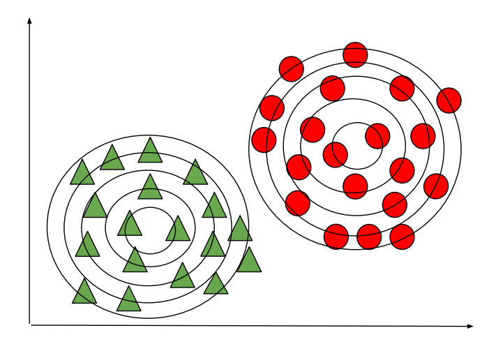
Generative Learning Algorithm (GDA)

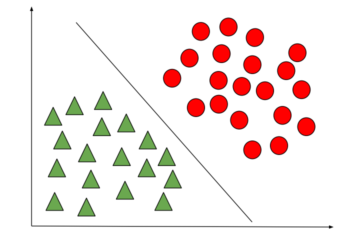
Discriminative Learning Algorithm

Let’s consider a binary classification problem such that all the data samples are IID (Independently and Identically distributed), therefore to calculate P(X|y) we can use Multivariate Gaussian Distribution to form a probability density function for each individual class. And to calculate P(y) or class prior for each class we can use Bernoulli distribution as all the data samples in binary classification can either take value 1 or 0.

Therefore, the probability distribution and class prior to a data sample can be defined using the general form of Gaussian and Bernoulli distribution respectively: 

[Tex]\\\\ In\hspace{1mm}the\hspace{1mm}above\hspace{1mm}equations:\\ \mu_0\hspace{1mm}is\hspace{1mm}the\hspace{1mm}mean\hspace{1mm} of\hspace{1mm} data\hspace{1mm} samples\hspace{1mm} corresponding\hspace{1mm} to\hspace{1mm} class\hspace{1mm}0\hspace{1mm}of\hspace{1mm}dimensions\hspace{1mm}\R^{n*1}\\\mu_1\hspace{1mm}is\hspace{1mm}the\hspace{1mm}mean\hspace{1mm} of\hspace{1mm} data\hspace{1mm} samples\hspace{1mm} corresponding\hspace{1mm} to\hspace{1mm} class\hspace{1mm} 1\hspace{1mm}of\hspace{1mm}dimensions\hspace{1mm}\R^{n*1}\\ \newline\Sigma\hspace{1mm}is \hspace{1mm}the \hspace{1mm}co-variance \hspace{1mm}matrix\hspace{1mm}of\hspace{1mm}dimensions\hspace{1mm}\R^{n*n}. \newline\hspace{1mm}\phi\hspace{1mm}is\hspace{1mm}the\hspace{1mm}probability\hspace{1mm}that\hspace{1mm}a\hspace{1mm}data\hspace{1mm}sample\hspace{1mm}belongs\hspace{1mm}to\hspace{1mm}class\hspace{1mm}y        \newline  [/Tex]

In order to view the probability distributions as a function of parameters mentioned above, we can define a Likelihood function which is equal to the product of probability distribution and class prior to each data sample (Taking product of the probabilities is reasonable as all the data samples are considered IID).

According to the principle of Maximum Likelihood estimation we have to choose the value of parameters in a way to maximize the probability function given in Eq 4. To do so instead of maximizing the Likelihood function we can maximize Log-Likelihood Function which is a strictly increasing function.

In the above equations, the function “1{condition}” is the indicator function which returns 1 if the condition is true else returns 0. For example, 1{y=1} will return 1 only when the class of that data sample is 1 else returns 0 similarly, in the case of 1{y=0} will return 1 only when the class of that data sample is 0 else it returns 0. 

The values of the parameters obtained can be plugged in Eq 1, 2, and 3 to find the probability distribution and class prior to all the data samples. These values obtained can be further multiplied to find the Likelihood function given in Eq 4. As mentioned earlier the likelihood function i.e P(X|y). P(y) can be plugged into the Bayes formula to predict P(y|X) (i.e predict the class ‘y‘ of a data sample for the given features ‘X‘). 

NOTE: The data samples in this model is considered to be IID which is an assumption made about the model, Gaussian Discriminant Analysis will perform poorly if the data is not a Gaussian distribution, therefore, it is always suggested visualizing the data to check if it has a normal distribution and if not attempts can be made to do so by using methods like log-transform etc. (Do not confuse Gaussian Discriminant Analysis with Gaussian Mixture model which is an unsupervised learning algorithm).

Therefore, Gaussian Discriminant Analysis works quite well for a small amount of data (say a few thousand examples) and can be more robust compared to Logistic Regression if our underlying assumptions about the distribution of the data are true 

Reference: http://cs229.stanford.edu/notes2020spring/cs229-notes2.pdf