Game Theory (Normal-form Game) | Set 6 (Graphical Method [2 X N] Game)
Last Updated :
01 Nov, 2023
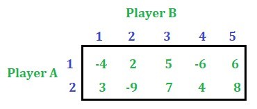
The payoff matrix of a
2 * N
game consists of
2 rows
and
N columns
. This article will discuss how to solve a
2 * N
game by graphical method. Consider the below 2 * 5 game:
Solution:
First check the saddle point of the game. This game has no saddle point.
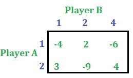
Step 1:
Reduce the size of the payoff matrix by applying
dominance property
, if it exists. This step is not compulsory. The size is being reduced to just simplify the problem. The game can be solved without reducing the size also. After reducing the above game with the help of dominance property we get the following game.
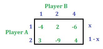
Step 2:
Let
x
be the probability of selection of alternative 1 by player A and
(1 – x)
be the probability of selection of alternative 2 by player A.
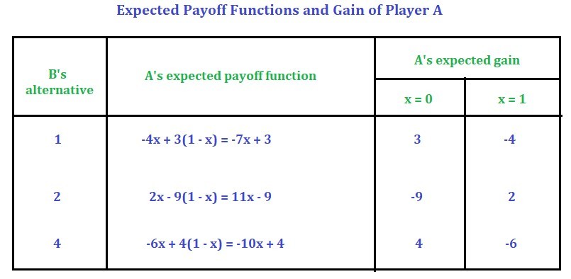
Derive the expected gain function of player A with respect to each of the alternatives of player B. To do this just multiply the column values of B’s alternative with its corresponding probability of selection of alternatives by player A. For example, the first alternative of player B is column number 1, so multiply
-4
with
x
and
3
with
(1 – x)
and add them then the expression obtained is the A’s expected payoff function. Similarly, the second alternative of player B is column number 2, so multiply
2
with
x
and
-9
with
(1 – x)
and add them. Similarly, the third alternative of player B is the column number 4, so multiply
-6
with
x
and
4
with
(1 – x)
and add them. Please refer the shown table.
Step 3:
Find the value of the gain when
x = 0
and
x = 1
. See the table below:
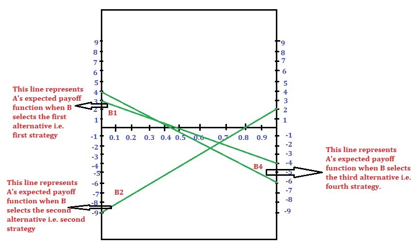
Step 4:
Now plot the gain function on a graph by assuming suitable scale. [Keep x on the x-axis and the gain on y-axis] If
B
selects the first alternative i.e. first strategy, when
x = 0
A’s expected gain is
3
and when
x = 1
A’s expected gain is
-4
. If
B
selects the second alternative i.e. second strategy, when
x = 0
A’s expected gain is
-9
and when
x = 1
A’s expected gain is
2
. If
B
selects the third alternative i.e. fourth strategy, when
x = 0
A’s expected gain is
4
and when
x = 1
A’s expected gain is
-6
. Using the above information plot the graph.
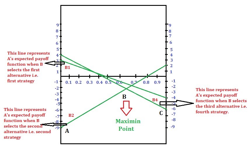
Step 5:
Find the highest intersection point in the lower boundary of the graph –>
Maximum point
as A is the
Maximin player
. The lower boundary is ABC. And the highest point among A, B and C is B. This intersection point B is called the
Maximin point
.
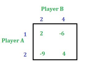
Step 6:
If the number of lines passing through the maximin point is only two, form 2 * 2 payoff matrix then solve the game as per
this article
. If not, identify any two lines with opposite slopes passing through that point. Form a 2 * 2 payoff matrix and then solve. This point will be discussed in the next article. Since we have two lines passing through this point, the payoff matrix using B1 and B2 alternatives are:
Now solve the game using the approach discussed in
this
article. Probabilities of Player A = [13/21, 8/21] Probabilities of Player B = [0, 10/21, 0, 11/21, 0] And the value of the game is -46/21
Like Article
Suggest improvement
Share your thoughts in the comments
Please Login to comment...