Freezing Panes in Excel to Lock Rows and Columns

Have you ever gotten lost in a big Excel file? Freeze Panes can help! It’s like a navigation tool that keeps important rows or columns visible while you scroll. Whether you’re new to Excel or a pro, mastering Freeze Panes will make your work easier.

In this article, we’ll learn about Freeze Panes in Excel. Let’s find out how Freeze Panes can make navigating through Excel files a breeze!

What are Freeze Panes in Excel?

Freeze Panes is a useful tool located in View Bar. In larger sheets, we have the data headers in the top rows and first columns. On scrolling down or to the right, these headers do not appear. The Excel Freeze Panes tool allows us to freeze the column/row or multiple columns/rows headings so that when we scroll down or move to the right to view the rest of the sheet, the rows/columns that are frozen remain on the screen. After freezing, below that row and column, a grey line appears to make the partition. 

In the Window group (View tab), we can see its variations:

Let’s discuss them and the other possibilities.

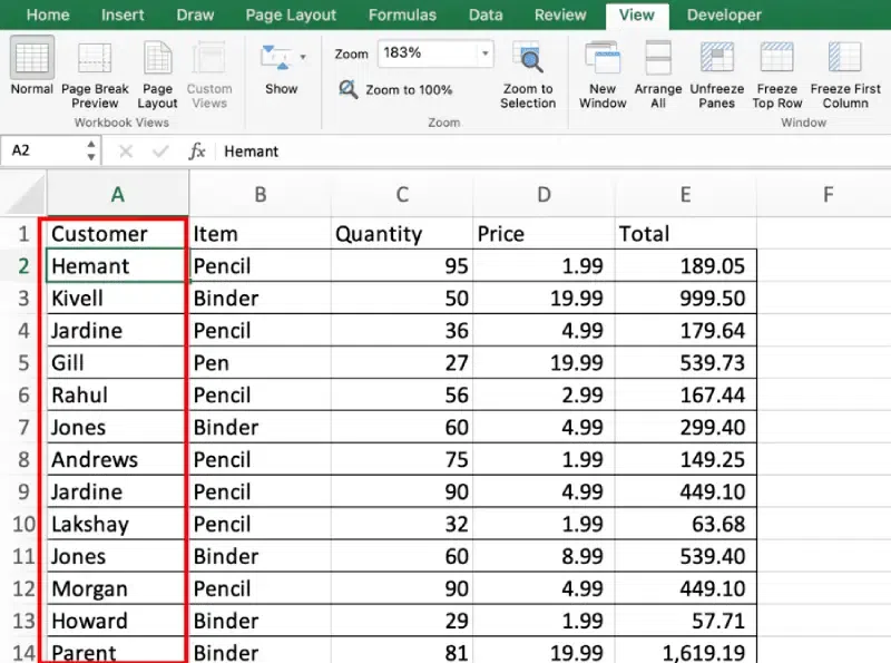
How to Freeze Top Row in Excel

On clicking Freeze Top Row under the Window section in the View tab, the First row gets frozen and on scrolling down, we can still see the top Row throughout the pages. 

Freezeing Top Row

After Scrolling also Freezed Pane is shown.

After Scrolling

How to Freeze First Column in Excel

On clicking Freeze First Column, the First Column gets frozen and on moving to the right, we can still see the First Column and can match the data values to the headers present in the first column. 

Freeze First Column

After Freezing first column

After Freezing first Column

Note: Freezing First Column and Top Row only freezes the one row/column to the screen. To freeze multiple, the Freeze Panes option is used.

How to Freeze Multiple Rows in Excel 

Step 1: Open Excel

Open your excel sheet whose row you want to freeze.

Step 2: Select the Cell

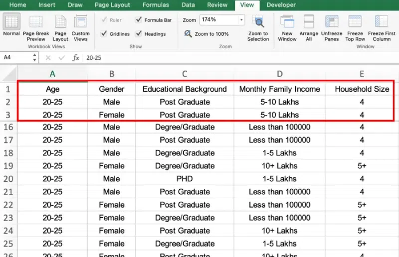
To freeze the multiple rows, select the cell in the first column(A) below the last row we want to freeze.

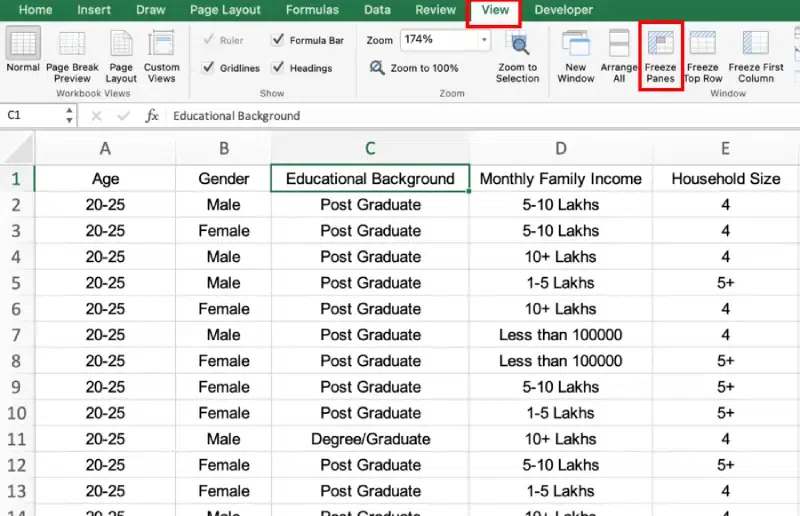
Step 3: Access View Tab and Select Freeze Panes

Go to the View Tab and then click on Freeze Panes. On scrolling down, frozen rows will stay fixed.

Access View Tab and Select Freeze Panes

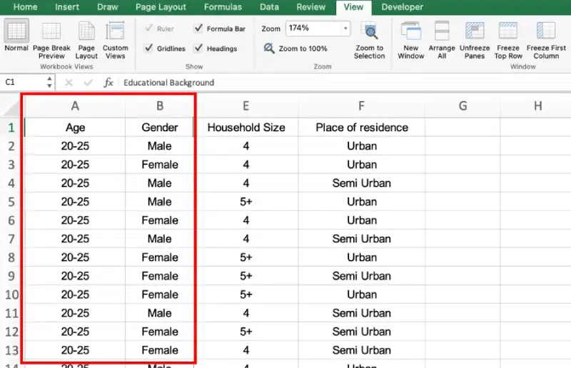
Cell A4 is selected so that the 3 rows above it get frozen.

Freezed first three Rows

How to Freeze Multiple Columns in Excel

Step 1: Open Excel

Open your excel sheet whose column you want to freeze.

Step 2: Select the Cell

To freeze the multiple columns, select the cell in the first row(1) right to the last column we want to freeze.

Step 3: Access View Tab and Click on Freeze Panes

Go to View Tab and then click on Freeze Panes. On moving to the right, frozen columns will stay fixed.

Access View Tab and Click on Freeze Panes

Cell C1 is selected, and after clicking on Freeze Panes, columns A and B get frozen.

After Freezing Columns

How to Freeze Cells in Excel

We can also Freeze Multiple Rows and Columns together as per requirement. The tool Freeze Panes will do the work for us.

Step 1: Open Excel

Open your excel sheet whose rows and columns you want to freeze.

Step 2: Select Cells

To freeze, we have to select the cell whose left columns need to be frozen and whose above rows need to be frozen.

Step 3: Access View Tab and Click on Freeze Panes

Go to View Tab and then click on Freeze Panes in the View Bar under Window Group. 

Access View Tab and Click on Freeze Panes

Cell C4 is selected to freeze the rows above it and the columns left to it. 

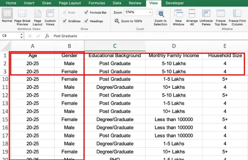
Freezing Rows

Freezing Columns you can see in the below image:

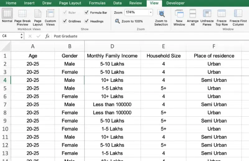
Freezing Columns

How to Unfreeze Panes in Excel

Unfreeze Panes is the tool used to unfreeze the formerly frozen row/column and the sheet gets back to normal view.

Step 1: Open Excel

Open your Excel Sheet whose freezer panes you want to Unfreeze.

Step 2: Access View Tab and Click on Unfreeze Panes

Go to the View Tab and Click on Unfreeze Panes Option under the Window Section to unfreeze already freezer rows or columns.
After freezing, the option Freeze Panes gets changed to Unfreeze Panes.

Access View Tab and Click on Unfreeze Panes

Conclusion

Freeze Panes in Excel helps you move around big spreadsheets better. It keeps important rows or columns visible while you scroll, making things easier to find. In the article, we learnt about freezing top row, first column and also about freezing multiple rows and columns in detail. Along with this we discussed how to unfreeze already locked cells.

Freezing Panes in Excel – FAQs

How do you freeze panes in Excel columns only?

To freeze panes in Excel for columns only:

1. Select the column to the right of the column you want to freeze.
2. Go to the View tab.
3. Click on Freeze Panes.
4. Choose “Freeze Panes” from the dropdown.

This will freeze all columns to the left of your selected column.

What are the three freeze pane options?

There are 3 options, Freeze Panes, Freeze First Row and Freeze First column

How do I freeze the first two rows in Excel?

To freeze the first two rows in Excel:

1. Click on the cell in row 3, column A.
2. Go to the View tab.
3. Click on Freeze Panes.
4. Select “Freeze Panes” from the dropdown menu.

This action freezes the first two rows of your worksheet.

What are the Shortcuts to Freeze pane in Excel?

You need to press ALT + W+ F to freeze panes in Excel. Further, you can select any one of your choice depending on what you want to freeze.

• Key F: To freeze both row and Column.
• Key C: To freeze first Column.
• Key R: To freeze top Row.

What are the view options in Excel?

There are three View Options in Excel :

1. Normal: Open Excel > View Tab > Normal.
2. Page Break: Open Excel > View Tab > Click Page Break Preview.
3. Page Layout: Open Excel > View Tab > Page Layout.