Fast R-CNN | ML

Before discussing Fast R-CNN, let’s look at the challenges faced by R-CNN.

• The training of R-CNN is very slow because each part of the model such as (CNN, SVM classifier, and bounding box) requires training separately and cannot be paralleled.
• Also, in R-CNN we need to forward and pass every region proposal through the Deep Convolution architecture (that’s up to ~2000 region proposals per image). That explains the amount of time taken to train this model
• The testing time of inference is also very high. It takes 49 seconds to test an image in R-CNN (along with selective search region proposal generation).

Fast R-CNN works to solve these problems. Let’s look at the architecture of Fast R-CNN.

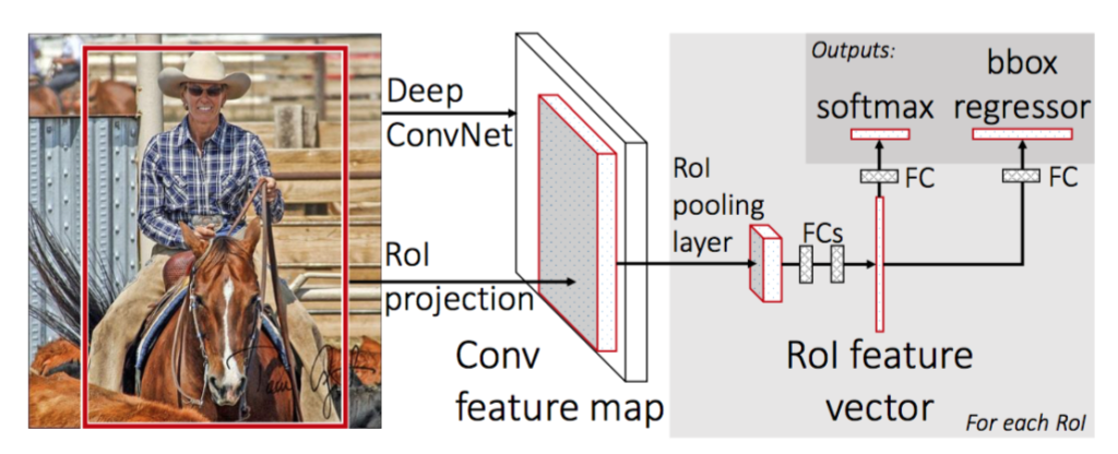
Fast R-CNN architecture

First, we generate the region proposal from a selective search algorithm. This selective search algorithm generates up to approximately 2000 region proposals. These region proposals (RoI projections) combine with input images passed into a CNN network. This CNN network generates the convolution feature map as output. Then for each object proposal, a Region of Interest (RoI) pooling layer extracts the feature vector of fixed length for each feature map. Every feature vector is then passed into twin layers of softmax classifier and Bbox regression for classification of region proposal and improve the position of the bounding box of that object.

CNN Network of Fast R-CNN

Fast R-CNN is experimented with three pre-trained ImageNet networks each with 5 max-pooling layers and 5-13 convolution layers (such as VGG-16). There are some changes proposed in this pre-trained network, These changes are:

• The network is modified in such a way that it two inputs the image and list of region proposals generated on that image.
• Second, the last pooling layer (here (7*7*512)) before fully connected layers needs to be replaced by the region of interest (RoI) pooling layer.
• Third, the last fully connected layer and softmax layer is replaced by twin layers of softmax classifier and K+1 category-specific bounding box regressor with a fully connected layer.

VGG-16 architecture

This CNN architecture takes the image (size = 224 x 224 x 3 for VGG-16) and its region proposal and outputs the convolution feature map (size = 14 x 14 x 512 for VGG-16).

Region of Interest (RoI) pooling:

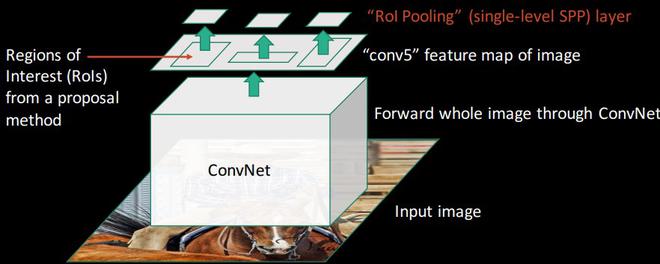
(Source: Fast R-CNN slides)

RoI pooling is a novel thing that was introduced in the Fast R-CNN paper. Its purpose is to produce uniform, fixed-size feature maps from non-uniform inputs (RoIs). It takes two values as inputs:

• A feature map was obtained from the previous CNN layer (14 x 14 x 512 in VGG-16).
• An N x 4 matrix represents regions of interest, where N is a number of RoIs, the first two represent the coordinates of the upper left corner of RoI and the other two represent the height and width of RoI denoted as (r, c, h, w).

Let’s consider we have 8*8 feature maps, we need to extract an output of size 2*2. We will follow the steps below.

Suppose we were given RoI’s left corner coordinates as (0, 3) and height, and width as (5, 7).

Now if we need to convert this region proposal into a 2 x 2 output block and we know that the dimensions of the pooling section do not perfectly divisible by output dimension. We take pooling such that it is fixed into 2 x 2 dimensions.

Now we apply the max pooling operator to select the maximum value from each of the regions that we divided into.

Max pooling output

Training and Loss Function

First, we take each training region of interest labeled with ground truth class u and ground truth bounding box v. Then we take the output generated by the softmax classifier and bounding box regressor and apply the loss function to them. We defined our loss function such that it takes into account both the classification and bounding box localization. This loss function is called multi-task loss. This is defined as follows:

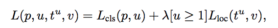
Multi-task Loss

where L_cls is classification loss, and L_loc is localization loss. lambda is a balancing parameter and u is a function (the value of u=0 for background, otherwise  u=1) to make sure that loss is only calculated when we need to define the bounding box. Here, L_cls is the log loss and L_loc is defined as

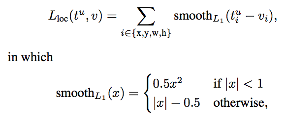
Loss function of Fast R-CNN model

Results and Conclusion

• Fast R-CNN provided state-of-the-art mAPs on VOC 2007, 2010, and 2012 datasets.
• It also improves detection time (84 vs 9.5 hrs) and training time (47 vs 0.32 seconds) considerably.

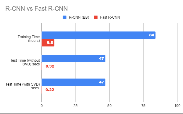
Performance comparison between R-CNN and Fast R-CNN

Advantages of Fast R-CNN over R-CNN

• The most important reason that Fast R-CNN is faster than R-CNN is that we don’t need to pass 2000 region proposals for every image in the CNN model. Instead, the convNet operation is done only once per image and a feature map is generated from it.
• Since the whole model is combined and trained in one go. So, there is no need for feature caching. That also decreases disk memory requirement while training.
• Fast R-CNN also improves mAP as compared to R-CNN on most of the classes of VOC 2007, 10, and 12 datasets.