Extract dominant colors of an image using Python

Let us see how to extract the dominant colors of an image using Python. Clustering is used in many real-world applications, one such real-world example of clustering is extracting dominant colors from an image. 

Any image consists of pixels, each pixel represents a dot in an image. A pixel contains three values and each value ranges between 0 to 255, representing the amount of red, green, and blue components. The combination of these forms an actual color of the pixel. To find the dominant colors, the concept of many k-means clustering is used. One important use of k-means clustering is to segment satellite images to identify surface features. 

Below shown satellite image contains the terrain of a river valley.

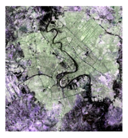
The terrain of the river valley

Various colors typically belong to different features, k-means clustering can be used to cluster them into groups which can then be identified into various surfaces like water, vegetation etc as shown below.

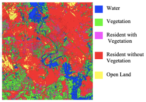
Clustered groups (water, open land, …)

Tools to find dominant colors

• matplotlib.image.imread – It converts JPEG image into a matrix which contains RGB values of each pixel.
• matplotlib.pyplot.imshow – This method would display colors of the cluster centers after k-means clustering performed on RGB values.

Lets now dive into an example, performing k-means clustering on the following image:

Example image

As it can be seen that there are three dominant colors in this image, a shade of blue, a shade of red and black.

Step 1 : The first step in the process is to convert the image to pixels using imread method of image class.

Python3

# Import image class of matplotlib
import matplotlib.image as img

# Read batman image and print dimensions
batman_image = img.imread('batman.png')
print(batman_image.shape)

Output :

(187, 295, 4)

The output is M*N*3 matrix where M and N are the dimensions of the image.

Step 2 : In this analysis, we are going to collectively look at all pixels regardless of their positions. So in this step, all the RGB values are extracted and stored in their corresponding lists. Once the lists are created, they are stored into the Pandas DataFrame, and then scale the DataFrame to get standardized values.

Python3

# Importing the modules
import pandas as pd
from scipy.cluster.vq import whiten

# Store RGB values of all pixels in lists r, g and b
r = []
g = []
b = []
for row in batman_image:
    for temp_r, temp_g, temp_b, temp in row:
        r.append(temp_r)
        g.append(temp_g)
        b.append(temp_b)

# only printing the size of these lists
# as the content is too big
print(len(r))
print(len(g))
print(len(b))

# Saving as DataFrame
batman_df = pd.DataFrame({'red': r,
                          'green': g,
                          'blue': b})

# Scaling the values
batman_df['scaled_color_red'] = whiten(batman_df['red'])
batman_df['scaled_color_blue'] = whiten(batman_df['blue'])
batman_df['scaled_color_green'] = whiten(batman_df['green'])

Output :

55165
55165
55165

Step 3 : Now, to find the number of clusters in k-means using the elbow plot approach . This is not an absolute method to find the number of clusters but helps in giving an indication about the clusters.

Elbow plot: a line plot between cluster centers and distortion (the sum of the squared differences between the observations and the corresponding centroid).

Below is the code to generate the elbow plot:

Python3

# Preparing data to construct elbow plot.
distortions = []
num_clusters = range(1, 7)  # range of cluster sizes

# Create a list of distortions from the kmeans function
for i in num_clusters:
    cluster_centers, distortion = kmeans(batman_df[['scaled_color_red',
                                                    'scaled_color_blue',
                                                    'scaled_color_green']], i)
    distortions.append(distortion)

# Create a data frame with two lists, num_clusters and distortions
elbow_plot = pd.DataFrame({'num_clusters': num_clusters,
                           'distortions': distortions})

# Create a line plot of num_clusters and distortions
sns.lineplot(x='num_clusters', y='distortions', data=elbow_plot)
plt.xticks(num_clusters)
plt.show()

Elbow plot is plotted as shown below :

Output :

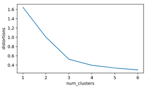
Elbow plot

It can be seen that a proper elbow is formed at 3 on the x-axis, which means the number of clusters is equal to 3 (there are three dominant colors in the given image).

Step 4 : The cluster centers obtained are standardized RGB values.

Standardized value = Actual value / Standard Deviation

Dominant colors are displayed using imshow() method, which takes RGB values scaled to the range of 0 to 1. To do so, you need to multiply the standardized values of the cluster centers with there corresponding standard deviations. Since the actual RGB values take the maximum range of 255, the multiplied result is divided by 255 to get scaled values in the range 0-1.

Python3

cluster_centers, _ = kmeans(batman_df[['scaled_color_red',
                                       'scaled_color_blue',
                                       'scaled_color_green']], 3)

dominant_colors = []

# Get standard deviations of each color
red_std, green_std, blue_std = batman_df[['red',
                                          'green',
                                          'blue']].std()

for cluster_center in cluster_centers:
    red_scaled, green_scaled, blue_scaled = cluster_center

    # Convert each standardized value to scaled value
    dominant_colors.append((
        red_scaled * red_std / 255,
        green_scaled * green_std / 255,
        blue_scaled * blue_std / 255
    ))

# Display colors of cluster centers
plt.imshow([dominant_colors])
plt.show()

Here is the resultant plot showing the three dominant colors of the given image.

Output :

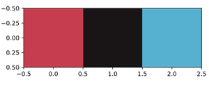
Plot showing dominant colors

Notice the three colors resemble the three that are indicative from visual inspection of the image.

Below is the full code without the comments :

Python3

import matplotlib.image as img
import matplotlib.pyplot as plt
from scipy.cluster.vq import whiten
from scipy.cluster.vq import kmeans
import pandas as pd

batman_image = img.imread('batman.jpg')

r = []
g = []
b = []
for row in batman_image:
    for temp_r, temp_g, temp_b, temp in row:
        r.append(temp_r)
        g.append(temp_g)
        b.append(temp_b)

batman_df = pd.DataFrame({'red': r,
                          'green': g,
                          'blue': b})

batman_df['scaled_color_red'] = whiten(batman_df['red'])
batman_df['scaled_color_blue'] = whiten(batman_df['blue'])
batman_df['scaled_color_green'] = whiten(batman_df['green'])

cluster_centers, _ = kmeans(batman_df[['scaled_color_red',
                                       'scaled_color_blue',
                                       'scaled_color_green']], 3)

dominant_colors = []

red_std, green_std, blue_std = batman_df[['red',
                                          'green',
                                          'blue']].std()

for cluster_center in cluster_centers:
    red_scaled, green_scaled, blue_scaled = cluster_center
    dominant_colors.append((
        red_scaled * red_std / 255,
        green_scaled * green_std / 255,
        blue_scaled * blue_std / 255
    ))

plt.imshow([dominant_colors])
plt.show()

Dominant Color Extraction using K-Means Clustering

• Import the necessary packages namely matplotlib.pyplot, matplotlib.image, and numpy
• The image file is loaded in the imread() function, which produces a NumPy array representing the image
• Using the shape attribute of the picture array, the width, height, and depth of the image are extracted
• The required number of colours for the output image is set in the variable n_colors. With 42 random states and n_colors clusters, a KMeans model is produced
• The model’s cluster_centers_ property is used to extract the cluster centres, which stand in for the image’s prominent colours.
• the cluster centres (colour palette) work with the image representation, they are transformed to the uint8 data type.
• Using plt.imshow(), the colour palette is presented as an image.
• The plot is then displayed using the plt.show() at the end. The number of dominating colours that appear in the output image can be changed by modifying the value of n_colors.

Python3

# Import the Packages
from sklearn.cluster import KMeans
import numpy as np
import matplotlib.pyplot as plt
import matplotlib.image as mpimg

# Load the image using mpimg.imread(). Use a raw string (prefix r) or escape the backslashes.
image = mpimg.imread(
    r'C:\Users\DELL\Desktop\INTERNSHIP\Mountain landscape.jpg')

# Get the dimensions (width, height, and depth) of the image
w, h, d = tuple(image.shape)

# Reshape the image into a 2D array, where each row represents a pixel
pixel = np.reshape(image, (w * h, d))

# Import the KMeans class from sklearn.cluster

# Set the desired number of colors for the image
n_colors = 18

# Create a KMeans model with the specified number of clusters and fit it to the pixels
model = KMeans(n_clusters=n_colors, random_state=42).fit(pixel)

# Get the cluster centers (representing colors) from the model
colour_palette = np.uint8(model.cluster_centers_)

# Display the color palette as an image
plt.imshow([colour_palette])

# Show the plot
plt.show()

Output: