Exponential Smoothing in R Programming

The Exponential Smoothing is a technique for smoothing data of time series using an exponential window function. It is a rule of the thumb method. Unlike simple moving average, over time the exponential functions assign exponentially decreasing weights. Here the greater weights are placed on the recent values or observations while the lesser weights are placed on the older values or observations. Among many window functions, in signal processing, the exponential smoothing function is generally applied to smooth data where it acts as a low pass filter in order to remove the high-frequency noise. This method is quite intuitive, generally can be applied on a wide or huge range of time series, and also is computationally efficient. In this article let’s discuss the exponential smoothing in R Programming. There are many types of exponential smoothing technique based on the trends and seasonality, which are as follows:

• Simple Exponential Smoothing
• Holt’s method
• Holt-Winter’s Seasonal method
• Damped Trend method

Before proceeding, one needs to see the replication requirements.

Replication Requirements of the Analysis in R

In R, the prerequisites of this analysis will be installing the required packages. We need to install the following two packages using the install.packages() command from the R console:

• fpp2 (with which the forecast package will be automatically loaded)
• tidyverse

Under the forecast package, we will get many functions that will enhance and help in our forecasting. In this analysis, we will be working with two data sets under the fpp2 package. These are the “goog” data set and the “qcement” data set. Now we need to load the required packages in our R Script using the library() function. After loading both the packages we will prepare our data set. For both the data set, we will divide the data into two sets, – train set and test set.

R

# loading the required packages
library(tidyverse)
library(fpp2)

# create training and testing set
# of the Google stock data
goog.train <- window(goog,
                     end = 900)
goog.test <- window(goog,
                    start = 901)

# create training and testing
# set of the AirPassengers data
qcement.train <- window(qcement,
                        end = c(2012, 4))
qcement.test <- window(qcement,
                       start = c(2013, 1))

Now we are ready to proceed with our analysis.

Simple Exponential Smoothing (SES)

The Simple Exponential Smoothing technique is used for data that has no trend or seasonal pattern. The SES is the simplest among all the exponential smoothing techniques. We know that in any type of exponential smoothing we weigh the recent values or observations more heavily rather than the old values or observations. The weight of each and every parameter is always determined by a smoothing parameter or alpha. The value of alpha lies between 0 and 1. In practice, if alpha is between 0.1 and 0.2 then SES will perform quite well. When alpha is closer to 0 then it is considered as slow learning since the algorithm is giving more weight to the historical data. If the value of alpha is closer to 1 then it is referred to as fast learning since the algorithm is giving the recent observations or data more weight. Hence we can say that the recent changes in the data will be leaving a greater impact on the forecasting.

In R, to perform the Simple Exponential Smoothing analysis we need to use the ses() function. To understand the technique we will see some examples. We will use the goog data set for SES.

Example 1:

In this example, we are setting alpha = 0.2 and also the forecast forward steps h = 100 for our initial model.

R

# SES in R
# loading the required packages
library(tidyverse)
library(fpp2)

# create training and validation
# of the Google stock data
goog.train <- window(goog, end = 900)
goog.test <- window(goog, start = 901)

# Performing SES on  the
# Google stock data
ses.goog <- ses(goog.train,
                alpha = .2,
                h = 100)
autoplot(ses.goog)

Output:

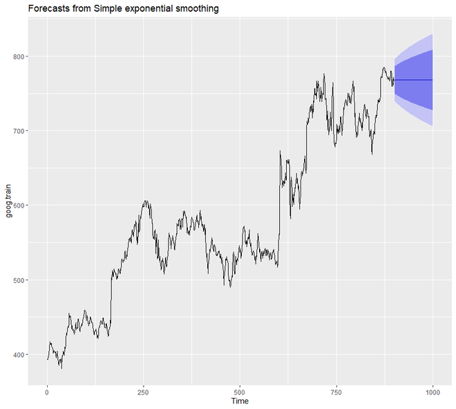
From the above output graph, we can notice that a flatlined estimate is projected towards the future by our forecast model. Hence we can say that from the data it is not capturing the present trend. Hence to correct this, we will be using the diff() function to remove the trend from the data.

Example 2:

R

# SES in R
# loading the required packages
library(tidyverse)
library(fpp2)

# create training and validation
# of the Google stock data
goog.train <- window(goog,
                     end = 900)
goog.test <- window(goog,
                    start = 901)

# removing the trend
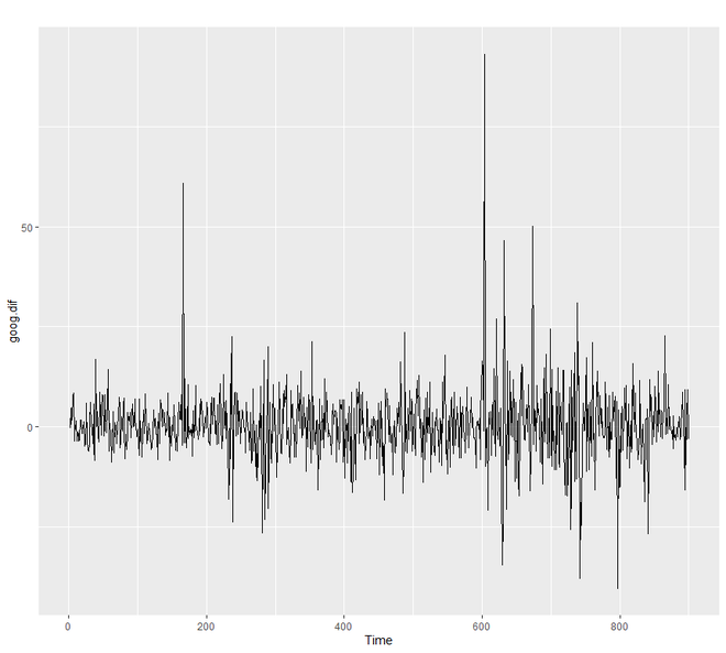
goog.dif <- diff(goog.train)
autoplot(goog.dif)

# reapplying SES on the filtered data
ses.goog.dif <- ses(goog.dif,
                    alpha = .2,
                    h = 100)
autoplot(ses.goog.dif)

Output:

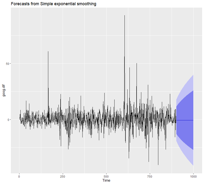
In order to understand the performance of our model, we need to compare our forecast with our validation or testing data set. Since our train data set was differenced, we need to form or create differenced validation or test set too. 

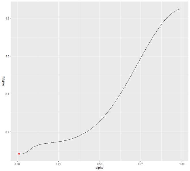
Example 3:

Here we are going to create a differenced validation set and then compare our forecast with the validation set. Here we are setting the value of alpha from 0.01-0.99 using the loop. We are trying to understand which level will be minimizing the RMSE test. We will see that 0.05 will be minimizing the most.

R

# SES in R
# loading the required packages
library(tidyverse)
library(fpp2)

# create training and validation
# of the Google stock data
goog.train <- window(goog,
                     end = 900)
goog.test <- window(goog,
                    start = 901)

# removing trend from test set
goog.dif.test <- diff(goog.test)
accuracy(ses.goog.dif, goog.dif.test)

# comparing our model
alpha <- seq(.01, .99, by = .01)
RMSE <- NA
for(i in seq_along(alpha)) {
  fit <- ses(goog.dif, alpha = alpha[i],
             h = 100)
  RMSE[i] <- accuracy(fit,
                      goog.dif.test)[2,2]
}

# convert to a data frame and
# identify min alpha value
alpha.fit <- data_frame(alpha, RMSE)
alpha.min <- filter(alpha.fit,
                    RMSE == min(RMSE))

# plot RMSE vs. alpha
ggplot(alpha.fit, aes(alpha, RMSE)) +
  geom_line() +
  geom_point(data = alpha.min,
             aes(alpha, RMSE),
             size = 2, color = "red")

Output:

                      ME     RMSE      MAE       MPE     MAPE      MASE        ACF1 Theil's U
Training set -0.01368221 9.317223 6.398819  99.97907 253.7069 0.7572009 -0.05440377        NA
Test set      0.97219517 8.141450 6.117483 109.93320 177.9684 0.7239091  0.12278141 0.9900678

Now, we will try to re-fit our forecast model for SES with alpha =0.05. We will notice the significant difference between alpha 0.02 and alpha=0.05.

Example 4:

R

# SES in R
# loading packages
library(tidyverse)
library(fpp2)

# create training and validation
# of the Google stock data
goog.train <- window(goog,
                     end = 900)
goog.test <- window(goog,
                    start = 901)

# removing trend
goog.dif <- diff(goog.train)

# refit model with alpha = .05
ses.goog.opt <- ses(goog.dif,
                    alpha = .05,
                    h = 100)

# performance eval
accuracy(ses.goog.opt, goog.dif.test)

# plotting results
p1 <- autoplot(ses.goog.opt) +
  theme(legend.position = "bottom")
p2 <- autoplot(goog.dif.test) +
  autolayer(ses.goog.opt, alpha = .5) +
  ggtitle("Predicted vs. actuals for
                 the test data set")

gridExtra::grid.arrange(p1, p2,
                        nrow = 1)

Output:

> accuracy(ses.goog.opt, goog.dif.test)
                      ME     RMSE      MAE       MPE     MAPE      MASE       ACF1 Theil's U
Training set -0.01188991 8.939340 6.030873 109.97354 155.7700 0.7136602 0.01387261        NA
Test set      0.30483955 8.088941 6.028383  97.77722 112.2178 0.7133655 0.12278141 0.9998811

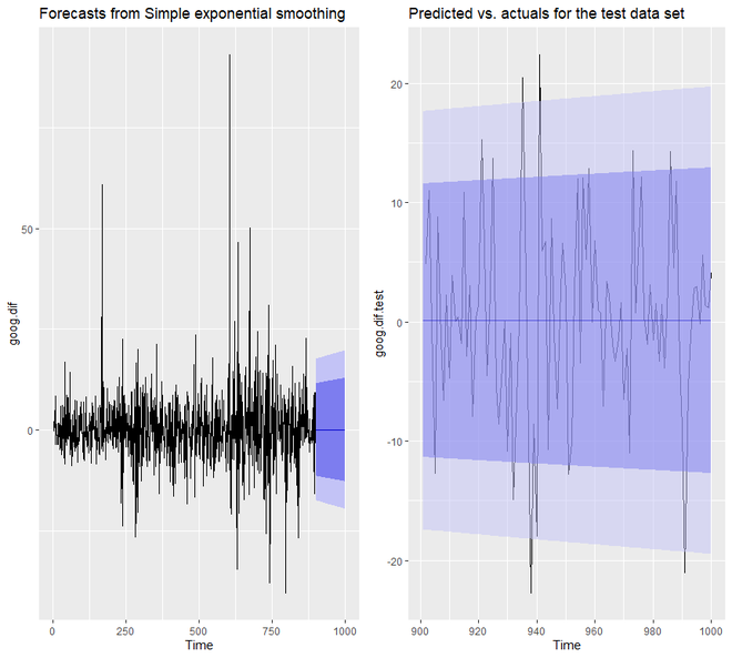
We will see that now the predicted confidence interval of our model is much narrower.

Holt’s Method

We have seen that in SES we had to remove the long-term trends to improve the model. But in Holt’s Method, we can apply exponential smoothing while we are capturing trends in the data. This is a technique that works with data having a trend but no seasonality. In order to make predictions on the data, the Holt’s Method uses two smoothing parameters, alpha, and beta, which correspond to the level components and trend components. 

In R, to apply the Holt’s Method we are going to use the holt() function. Again we will understand the working principle of this technique using some examples. We are going to use the goog data set again.

Example 1:

R

# holt's method in R

# loading packages
library(tidyverse)
library(fpp2)

# create training and validation
# of the Google stock data
goog.train <- window(goog,
                     end = 900)
goog.test <- window(goog,
                    start = 901)

# applying holt's method on
# Google stock Data
holt.goog <- holt(goog.train,
                  h = 100)
autoplot(holt.goog)

Output:

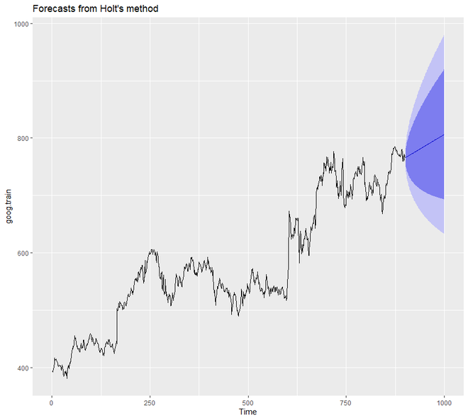
In the above example, we did not set the value of alpha and beta manually. But we can do so. However, if we do mention any value for alpha and beta then automatically the holt() function will identify the optimal value. In this case, if the value of the alpha is 0.9967 then it indicates fast learning and if the value of beta is 0.0001 then it indicates slow learning of the trend.

Example 2:

In this example, we are going to set the value of alpha and beta. Also, we are going to see the accuracy of the model.

R

# holt's method in R

# loading the packages
library(tidyverse)
library(fpp2)

# create training and validation
# of the Google stock data
goog.train <- window(goog,
                     end = 900)
goog.test <- window(goog,
                    start = 901)

# holt's method
holt.goog$model

# accuracy of the model
accuracy(holt.goog, goog.test)

Output:

Holt's method 

Call:
 holt(y = goog.train, h = 100) 

  Smoothing parameters:
    alpha = 0.9999 
    beta  = 1e-04 

  Initial states:
    l = 401.1276 
    b = 0.4091 

  sigma:  8.8149

     AIC     AICc      BIC 
10045.74 10045.81 10069.75 

> accuracy(holt.goog, goog.test)
                       ME      RMSE       MAE         MPE     MAPE     MASE       ACF1 Theil's U
Training set -0.003332796  8.795267  5.821057 -0.01211821 1.000720 1.002452 0.03100836        NA
Test set      0.545744415 16.328680 12.876836  0.03013427 1.646261 2.217538 0.87733298  2.024518

The optimal value i.e. beta =0.0001 is used to remove errors from the training set. We can tune our beta to this optimal value. 

Example 3:

Let us try to find the optimal value of beta through a loop ranging from 0.0001 to 0.5 that will minimize the RMSE test. We will see that 0.0601 will be the value of beta that will dip RMSE.

R

# holts method in R
# loading the package
library(tidyverse)
library(fpp2)

# create training and validation
# of the Google stock data
goog.train <- window(goog,
                     end = 900)
goog.test <- window(goog,
                    start = 901)

# identify optimal alpha parameter
beta <- seq(.0001, .5, by = .001)
RMSE <- NA
for(i in seq_along(beta)) {
  fit <- holt(goog.train,
              beta = beta[i],
              h = 100)
  RMSE[i] <- accuracy(fit,
                      goog.test)[2,2]
}

# convert to a data frame and
# identify min alpha value
beta.fit <- data_frame(beta, RMSE)
beta.min <- filter(beta.fit,
                   RMSE == min(RMSE))

# plot RMSE vs. alpha
ggplot(beta.fit, aes(beta, RMSE)) +
  geom_line() +
  geom_point(data = beta.min,
             aes(beta, RMSE),
             size = 2, color = "red")

Output:

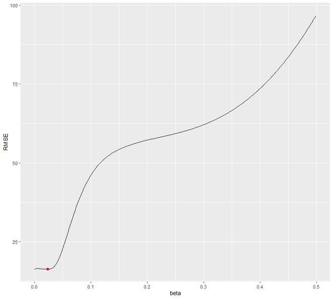
Now let us refit the model with the obtained optimal value of beta. 

Example 4:

We are going to set the optimal value of beta and also compare the predictive accuracy with our original model.

R

# loading the package
library(tidyverse)
library(fpp2)

# create training and validation
# of the Google stock data
goog.train <- window(goog,
                     end = 900)
goog.test <- window(goog,
                    start = 901)

holt.goog <- holt(goog.train,
                  h = 100)

# new model with optimal beta
holt.goog.opt <- holt(goog.train,
                      h = 100,
                      beta = 0.0601)

# accuracy of first model
accuracy(holt.goog, goog.test)

# accuracy of new optimal model
accuracy(holt.goog.opt, goog.test)

p1 <- autoplot(holt.goog) +
  ggtitle("Original Holt's Model") +
  coord_cartesian(ylim = c(400, 1000))

p2 <- autoplot(holt.goog.opt) +
  ggtitle("Optimal Holt's Model") +
  coord_cartesian(ylim = c(400, 1000))

gridExtra::grid.arrange(p1, p2,
                        nrow = 1)

Output:

> accuracy(holt.goog, goog.test)
                       ME      RMSE       MAE         MPE     MAPE     MASE       ACF1 Theil's U
Training set -0.003332796  8.795267  5.821057 -0.01211821 1.000720 1.002452 0.03100836        NA
Test set      0.545744415 16.328680 12.876836  0.03013427 1.646261 2.217538 0.87733298  2.024518

> accuracy(holt.goog.opt, goog.test)
                      ME      RMSE       MAE          MPE     MAPE     MASE        ACF1 Theil's U
Training set -0.01493114  8.960214  6.058869 -0.005524151 1.039572 1.043406 0.009696325        NA
Test set     21.41138275 28.549029 23.841097  2.665066997 2.988712 4.105709 0.895371665  3.435763

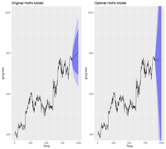
We will notice that the optimal model compared to the original model is much more conservative. Also, the confidence interval of the optimal model is much more extreme. 

Holt-Winter’s Seasonal Method

The Holt-Winter’s Seasonal method is used for data with both seasonal patterns and trends. This method can be implemented either by using Additive structure or by using the Multiplicative structure depending on the data set. The Additive structure or model is used when the seasonal pattern of data has the same magnitude or is consistent throughout, while the Multiplicative structure or model is used if the magnitude of the seasonal pattern of the data increases over time. It uses three smoothing parameters,- alpha, beta, and gamma.

In R, we use the decompose() function to perform this kind of exponential smoothing. We will be using the qcement data set to study the working of this technique.

Example 1:

R

# Holt-Winter's method in R
# loading packages
library(tidyverse)
library(fpp2)

# create training and validation
# of the AirPassengers data
qcement.train <- window(qcement,
                        end = c(2012, 4))
qcement.test <- window(qcement,
                       start = c(2013, 1))

# applying holt-winters
# method on qcement
autoplot(decompose(qcement))

Output:

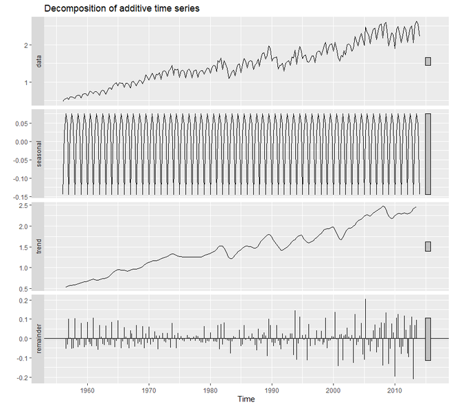
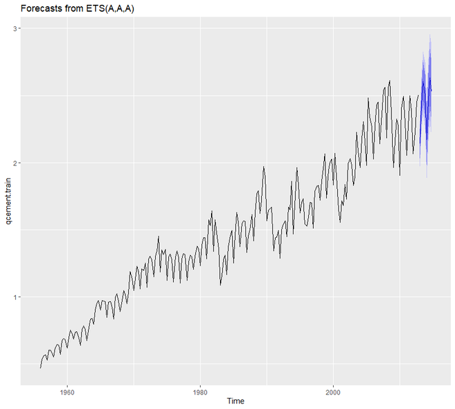
In order to create an Additive Model that deals with error, trend, and seasonality, we are going to use the ets() function. Out of the 36 models, the ets() chooses the best additive model. For additive model, the model parameter of ets() will be ‘AAA’.

Example 2:

R

# loading package
library(tidyverse)
library(fpp2)

# create training and validation
# of the AirPassengers data
qcement.train <- window(qcement,
                        end = c(2012, 4))
qcement.test <- window(qcement,
                       start = c(2013, 1))

# applying ets
qcement.hw <- ets(qcement.train,
                  model = "AAA")
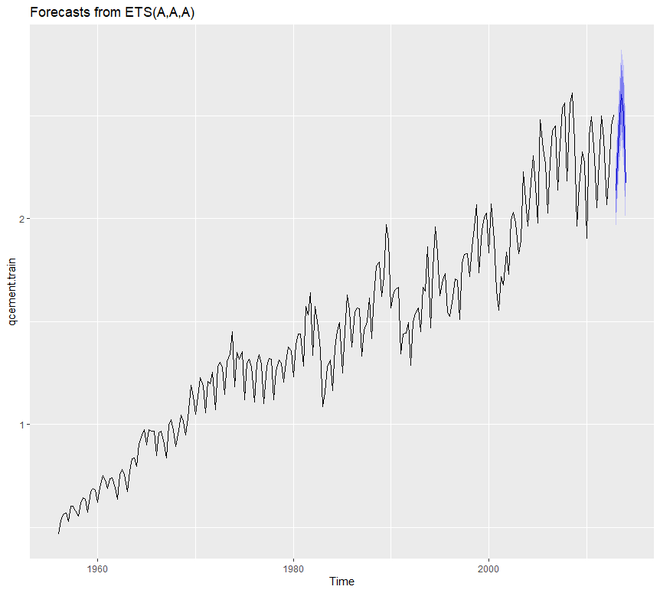
autoplot(forecast(qcement.hw))

Output:

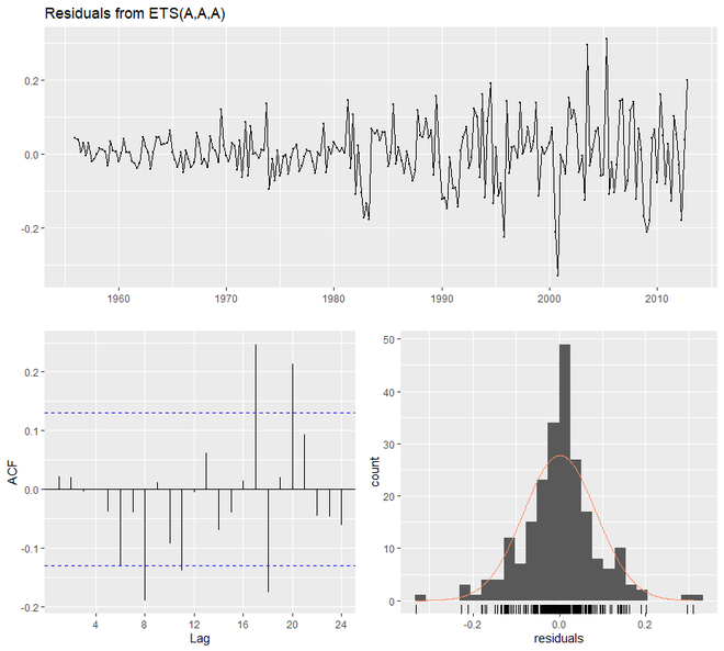
Now we will assess our model and summarize the smoothing parameters. We will also check the residuals and find out the accuracy of our model.

Example 3:

R

# additive model
# loading packages
library(tidyverse)
library(fpp2)

# create training and validation
# of the AirPassengers data
qcement.train <- window(qcement,
                        end = c(2012, 4))
qcement.test <- window(qcement,
                       start = c(2013, 1))

qcement.hw <- ets(qcement.train, model = "AAA")

# assessing our model
summary(qcement.hw)
checkresiduals(qcement.hw)

# forecast the next 5 quarters
qcement.f1 <- forecast(qcement.hw,
                       h = 5)

# check accuracy
accuracy(qcement.f1, qcement.test)

Output:

> summary(qcement.hw)
ETS(A,A,A) 

Call:
 ets(y = qcement.train, model = "AAA") 

  Smoothing parameters:
    alpha = 0.6418 
    beta  = 1e-04 
    gamma = 0.1988 

  Initial states:
    l = 0.4511 
    b = 0.0075 
    s = 0.0049 0.0307 9e-04 -0.0365

  sigma:  0.0854

     AIC     AICc      BIC 
126.0419 126.8676 156.9060 

Training set error measures:
                      ME       RMSE       MAE          MPE     MAPE      MASE       ACF1
Training set 0.001463693 0.08393279 0.0597683 -0.003454533 3.922727 0.5912949 0.02150539

> checkresiduals(qcement.hw)

    Ljung-Box test

data:  Residuals from ETS(A,A,A)
Q* = 20.288, df = 3, p-value = 0.0001479

Model df: 8.   Total lags used: 11

> accuracy(qcement.f1, qcement.test)
                      ME       RMSE        MAE          MPE     MAPE      MASE        ACF1 Theil's U
Training set 0.001463693 0.08393279 0.05976830 -0.003454533 3.922727 0.5912949  0.02150539        NA
Test set     0.031362775 0.07144211 0.06791904  1.115342984 2.899446 0.6719311 -0.31290496 0.2112428

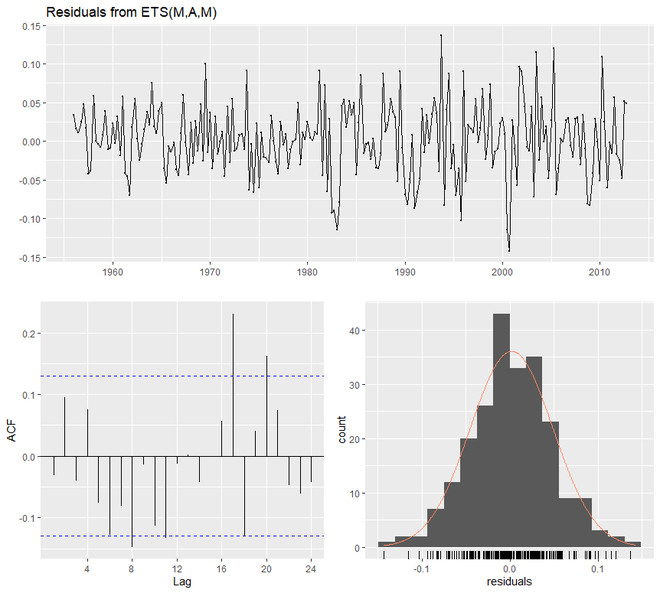
Now we are going to see how the Multiplicative model works using ets(). For that purpose, the model parameter of ets() will be ‘MAM’.

Example 4:

R

# multiplicative model in R
# loading package
library(tidyverse)
library(fpp2)

# create training and validation
# of the AirPassengers data
qcement.train <- window(qcement,
                        end = c(2012, 4))
qcement.test <- window(qcement,
                       start = c(2013, 1))

# applying ets
qcement.hw2 <- ets(qcement.train,
                   model = "MAM")
checkresiduals(qcement.hw2)

Output:

> checkresiduals(qcement.hw2)

    Ljung-Box test

data:  Residuals from ETS(M,A,M)
Q* = 23.433, df = 3, p-value = 3.281e-05

Model df: 8.   Total lags used: 11

Here we will optimize the gamma parameter in order to minimize the error rate. The value of gamma will be 0.21. Along with that, we are going to find out the accuracy and also plot the predictive values. 

Example 5:

R

# Holt winters model in R
# loading packages
library(tidyverse)
library(fpp2)

# create training and validation
# of the AirPassengers data
qcement.train <- window(qcement,
                        end = c(2012, 4))
qcement.test <- window(qcement,
                       start = c(2013, 1))

qcement.hw <- ets(qcement.train,
                  model = "AAA")

# forecast the next 5 quarters
qcement.f1 <- forecast(qcement.hw,
                       h = 5)

# check accuracy
accuracy(qcement.f1, qcement.test)

gamma <- seq(0.01, 0.85, 0.01)
RMSE <- NA

for(i in seq_along(gamma)) {
  hw.expo <- ets(qcement.train,
                 "AAA",
                 gamma = gamma[i])
  future <- forecast(hw.expo,
                     h = 5)
  RMSE[i] = accuracy(future,
                     qcement.test)[2,2]
}

error <- data_frame(gamma, RMSE)
minimum <- filter(error,
                  RMSE == min(RMSE))
ggplot(error, aes(gamma, RMSE)) +
  geom_line() +
  geom_point(data = minimum,
             color = "blue", size = 2) +
  ggtitle("gamma's impact on
            forecast errors",
  subtitle = "gamma = 0.21 minimizes RMSE")

# previous model with additive
# error, trend and seasonality
accuracy(qcement.f1, qcement.test)


# new model with
# optimal gamma parameter
qcement.hw6 <- ets(qcement.train,
                   model = "AAA",
                   gamma = 0.21)
qcement.f6 <- forecast(qcement.hw6,
                       h = 5)
accuracy(qcement.f6, qcement.test)

# predicted values
qcement.f6
autoplot(qcement.f6)

Output:

> accuracy(qcement.f1, qcement.test)
                      ME       RMSE        MAE          MPE     MAPE      MASE        ACF1 Theil's U
Training set 0.001463693 0.08393279 0.05976830 -0.003454533 3.922727 0.5912949  0.02150539        NA
Test set     0.031362775 0.07144211 0.06791904  1.115342984 2.899446 0.6719311 -0.31290496 0.2112428

> accuracy(qcement.f6, qcement.test)
                       ME       RMSE        MAE        MPE     MAPE      MASE        ACF1 Theil's U
Training set -0.001312025 0.08377557 0.05905971 -0.2684606 3.834134 0.5842847  0.04832198        NA
Test set      0.033492771 0.07148708 0.06775269  1.2096488 2.881680 0.6702854 -0.35877010 0.2202448

> qcement.f6
        Point Forecast    Lo 80    Hi 80    Lo 95    Hi 95
2013 Q1       2.134650 2.025352 2.243947 1.967494 2.301806
2013 Q2       2.427828 2.299602 2.556055 2.231723 2.623934
2013 Q3       2.601989 2.457284 2.746694 2.380681 2.823296
2013 Q4       2.505001 2.345506 2.664496 2.261075 2.748927
2014 Q1       2.171068 1.987914 2.354223 1.890958 2.451179

Damping Method in R

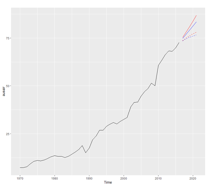
The damping method uses the damping coefficient phi to estimate more conservatively the predicted trends. The value of phi lies between 0 and 1. If we believe that our additive and multiplicative model is going to be a flat line then chance are there that it is damped. To understand the working principle of damping forecasting we will use the fpp2::ausair data set where we will create many models and try to have much more conservative trend lines,

Example:

R

# Damping model in R

# loading the packages
library(tidyverse)
library(fpp2)

# holt's linear (additive) model
fit1 <- ets(ausair, model = "ZAN",
            alpha = 0.8, beta = 0.2)
pred1 <- forecast(fit1, h = 5)

# holt's linear (additive) model
fit2 <- ets(ausair, model = "ZAN",
            damped = TRUE, alpha = 0.8,
            beta = 0.2, phi = 0.85)
pred2 <- forecast(fit2, h = 5)

# holt's exponential
# (multiplicative) model
fit3 <- ets(ausair, model = "ZMN",
            alpha = 0.8, beta = 0.2)
pred3 <- forecast(fit3, h = 5)

# holt's exponential
# (multiplicative) model damped
fit4 <- ets(ausair, model = "ZMN",
            damped = TRUE,
            alpha = 0.8, beta = 0.2,
            phi = 0.85)
pred4 <- forecast(fit4, h = 5)

autoplot(ausair) +
  autolayer(pred1$mean,
            color = "blue") +
  autolayer(pred2$mean,
            color = "blue",
            linetype = "dashed") +
  autolayer(pred3$mean,
            color = "red") +
  autolayer(pred4$mean,
            color = "red",
            linetype = "dashed")

Output: