Exploratory Data Analysis in Julia
Last Updated :
09 Nov, 2022
Exploratory Data Analysis (EDA) is used for achieving a better understanding of data in terms of its main features, the significance of various variables, and the inter-variable relationships. The First step is to explore the dataset.
Methods to explore the given dataset in Julia:
- Using data tables and applying statistics
- Using Visual Plotting techniques on the data
Using data tables and applying statistics
Step 1: Install DataFrames Package
For using data tables in Julia, a data structure called Dataframe is used. DataFrame can handle multiple operations without compromising on Speed and Scalability.
Dataframes package can be installed using the following command:
using Pkg
Pkg.add(“DataFrames”)
Step 2: Download the Dataset
For data analysis, we have used the Iris dataset. It is easily available online.
Step 3: Import Necessary Packages and the Dataset
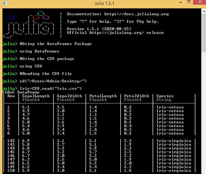
Let’s first import our DataFrames Package, CSV Package, and load the Iris.csv file of the data set:
Julia
using DataFrames
using CSV
Iris = CSV.read(“Iris.csv”)
|
Output:
Step 4: Quick Data Exploration
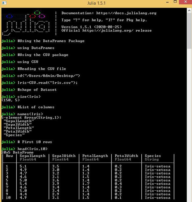
Preliminary exploration can be performed on the dataset such as identifying the shape of the dataset using the size function, list of columns using the names function, first n rows using the head function.
Example:
Julia
using DataFrames
using CSV
Iris = CSV.read(“Iris.csv”);
size(Iris)
names(Iris)
head(Iris, 10)
|
Output:
Indexing in a dataframe
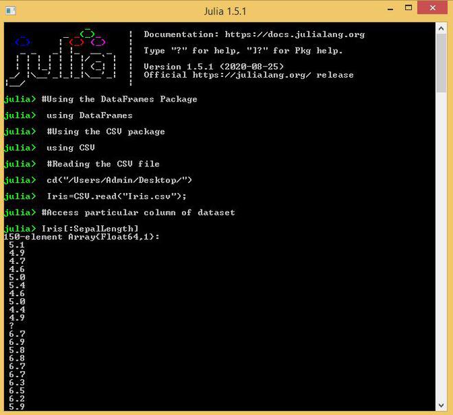
Dataframe_name[:column_name] is a basic indexing technique to access a particular column of the data frame.
Example:
Julia
using DataFrames
using CSV
Iris = CSV.read(“Iris.csv”);
Iris[: SepalLength]
|
Output:
Describe Function
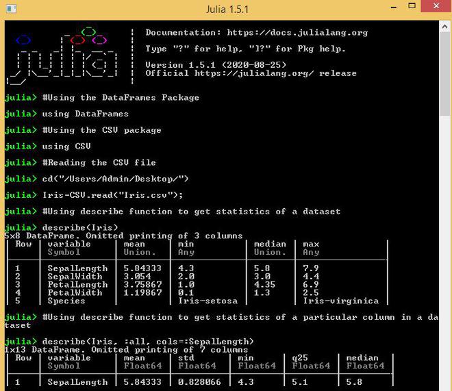
Describe function is used to present the mean, median, minimum, maximum, quartiles, etc of the dataset.
Example:
Julia
using DataFrames
using CSV
Iris = CSV.read(“Iris.csv”);
describe(Iris)
describe(Iris, :all, cols=:SepalLength)
|
Output:
Using Visual Plotting techniques on the data
Visual Exploration in Julia can be achieved with the help of various plotting libraries such as Plots, StatPlots, and Pyplot.
Plots: It is a high-level plotting package that interfaces other plotting packages called ‘back-ends‘. They behave like the graphics engines that generate the graphics. It has a simple and consistent interface.
StatPlots: It is a supporting package used with Plots package consisting of statistical recipes for various concepts and types.
PyPlot: It is used to work with matplotlib library of Python in Julia.
The above-mentioned libraries can be installed using the following commands:
Pkg.add(“Plots”)
Pkg.add(“StatPlots”)
Pkg.add(“PyPlot”)
Distribution analysis
The distribution of variables in Julia can be performed using various plots such as histogram, boxplot, scatterplot, etc.
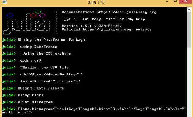
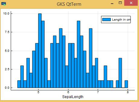
Let’s start by plotting the histogram of SepalLength:
Example:
Julia
using DataFrames
using CSV
Iris = CSV.read("Iris.csv");
using Plots
Plots.histogram(Iris[:SepalLength],
bins = 50, xlabel = "SepalLength",
labels = "Length in cm")
|
Output:
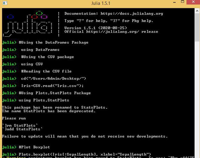
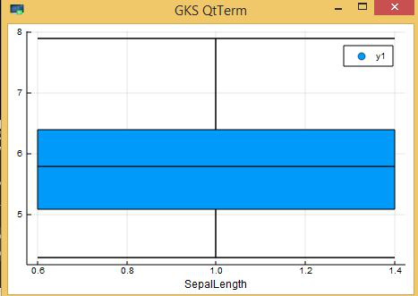
Next, we look at box plots to understand the distributions. Box plot for SepalLength can be plotted by:
Example:
Julia
using DataFrames
using CSV
Iris = CSV.read("Iris.csv");
using Plots, StatPlots
Plots.boxplot(Iris[:SepalLength],
xlabel = "SepalLength")
|
Output:
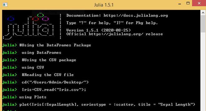
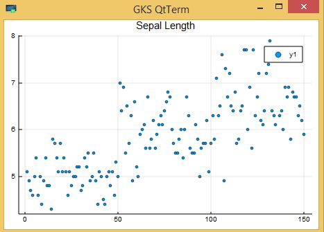
Next, we look at Scatter plot to understand the distributions. Scatter plot for SepalLength can be plotted by:
Example:
Julia
using DataFrames
using CSV
Iris = CSV.read("Iris.csv");
using Plots
plot(Iris[:SepalLength],
seriestype = :scatter,
title = "Sepal Length")
|
Output:
Like Article
Suggest improvement
Share your thoughts in the comments
Please Login to comment...