Excel CHOOSE Function with Array

We often use the CHOOSE function in Excel to pick something from a list. In this article, we’ll see how to use CHOOSE with a bunch of things (we call it an array) to do various stuff in Excel. This array can be either many cells we put into the function or many things we get from the function.

What is CHOOSE Function with Array in Excel

The Excel CHOOSE function stands out as a powerful tool that enables you to retrieve the values or references from an array based on a specified position. This guide retrieves values or references from an array based on a specified position. In this context, “array” refers to the scenario where we either provide multiple cells as input within the function or obtain multiple results by using the function.

Syntax of CHOOSE Function

=CHOOSE (index_num, value1, [value2], …)

Arguments:  

• index_num: The value to choose.
• value1: The first value from which to choose.
• value2 [optional]: The second value from which to choose.
• index_num: It is the first argument for the CHOOSE function and it refers to the position of an array.

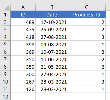
Sample Data: In the Sales Table, we have given Products_Id.  We use Excel CHOOSE() to fill in the Actual product name in the next column (Column – D).

How to Use CHOOSE Function with Array in Excel

You can learn how to use CHOOSE Function with Array in Excel by the following methods:

• Return Single Value in Excel Using CHOOSE Function with Array
• Apply CHOOSE Function with Array to Return Multiple Values in Excel
• Assign CHOOSE Function with Array to Retuen a Cell Reference
• Apply CHOOSE Function with Array for Left VLOOKUP

How to Return Single Value in Excel Using CHOOSE Function With Array

Step 1: Type Products in Cell D1

Type “Products” in cell D1

Step 2: Use CHOOSE Function

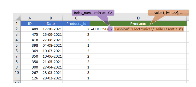
Write a CHOOSE function in cell D2  

=CHOOSE(C2,”Fashion”,”Electronics”,”Daily Essentials”)

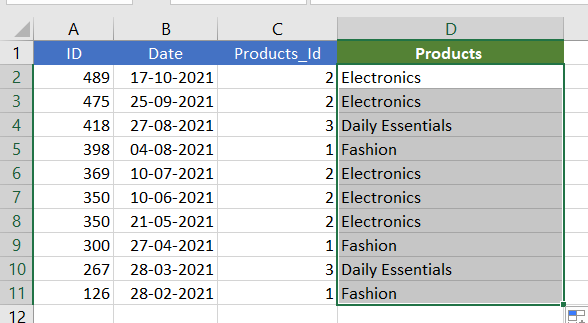
Step 3: Drag the Formula

Select cell D2 and drag till cell D11

How to Apply CHOOSE Function with Array to Return Multiple Values in Excel

We have a Dataset (A1:D11) in Excel Containing the Products with their ID. We need to pick a ID along with the products_ID and Product Name. Here we will use the CHOOSE Function in Excel with the array to return these multiples values. By applying the formula of this method we can get the values in a row even if they are in a column.

Step 1: Select the Cell

Select the cell where you need the result.

Step 2: Enter the Formula in the Cell

Enter the Formula in the Cell “=CHOOSE({1,2,3},

Step 3: Preview the Result

Drag the Formula to all the cells and see the Result.

How to Apply CHOOSE Function with Array to Returning a cell reference

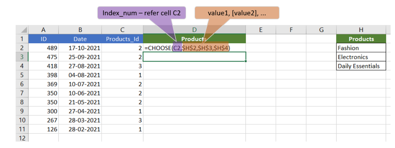
Step 1: Type “Products” in cell D1

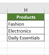
Step 2: Create a Product table (unique list of Products)

Step 3: Write a CHOOSE function in cell D2

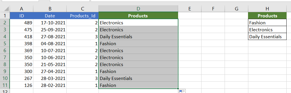
=CHOOSE(C2, $H$2,$H$3,$H$4)

Step 4: Select cell D2 and drag till cell D11

How to Use CHOOSE Function with Array for Left VLOOKUP

When we want to find something in Excel using the VLOOKUP function, it typically only searches in the leftmost column. However, sometimes we need to look in other columns. We can solve this by using the CHOOSE function together with an array.

Here’s a simple example to understand this:

Step 1: Enter the Data Set

We have a dataset that lists product names and their corresponding IDs (in cells B2:D11).

Step 2: Search for the Value

Let’s say we want to find the product of the Product_ID “418” and place it in cell F5.

Step 3: Enter the VLOOKUP Formula

First, we try using VLOOKUP alone, but it has a limitation as it only searches the leftmost column.

Step 4: Use VLOOKUP and CHOOSE Function

Then, we’ll show you how to overcome this limitation by combining the CHOOSE function with VLOOKUP.

This combination allows us to search for information in columns other than the leftmost one.

Formula :=VLOOKUP(F4,CHOOSE({1,2},A4:A8,C4:C8),2,FALSE)

FAQs

What is the Purpose of Excel’s CHOOSE function with an array?

The CHOOSE function with an array in Excel serves the purpose of selecting a value or reference from a list of options based on a numeric index, It also allows users to dynamically retrieve data from an array and is particularly useful for scenarios where you need to display different values based on specific conditions.

How does the CHOOSE function with an array work?

The CHOOSE function with an array operates by using a numeric index to determine the position of the value or reference within the array. The function takes the index_num as its first argument and subsequent arguments represent the values or references in the array. The value/reference corresponding to the specified index_num is returned by the function.

What are the limitations of using the CHOOSE function with an array?

CHOOSE function is a powerful tool, but it has a limitation in terms of the number of values/references that can be included as arguments. Excel supports a maximum of 254 arguments within the CHOOSE function.

Q4: Can we use cell references as arguments in the CHOOSE function with an array?

Yes, you can use cell references as arguments in the CHOOSE function with an array. This allows you to create a dynamic formula that adapts to changes in the referenced cells.