How to Create Excel Pivot Table Calculated Field with Examples
Last Updated :
06 Dec, 2023
You can add calculated fields to a pivot table using your own unique algorithms that add up to other pivot fields. A calculated field has some restrictions, but it gives the pivot tables in your Excel worksheet a strong tool.
What is a Pivot Table Calculated Field in Excel
“Pivot Table calculated field” is an option to include more data or calculations in the pivot table. Often, we need to add our own custom calculations that can refer to other fields in the data set for our reports.
In the below examples, we create a sales report by-product with an additional column “Sales Differences” [2020_Sales – 2019_Sales]. The calculated field “Sales Differences” calculation refers to other fields in the dataset [subtract 2019_Sales from 2020_Sales].
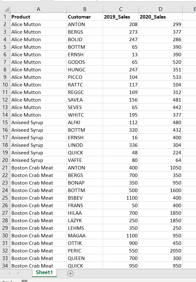
Example: We have a data set in four columns “Product”, ”Customer”, “2019_Sales” and “2020_Sales” as below
How to Create a Pivot Table in Excel
Follow the below steps to create a pivot table
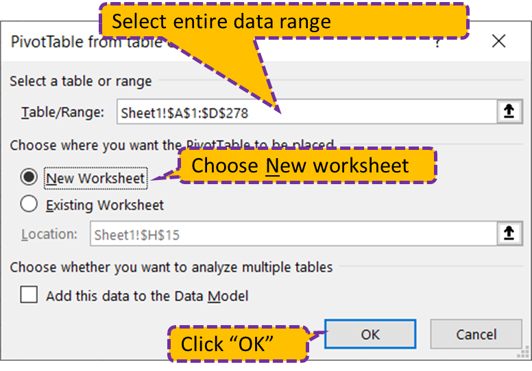
Step 1: Select Insert >> Pivot >> From Table/Range (Img1) to pop-up “Pivot Table from table or range” dialogue box (Img 2).
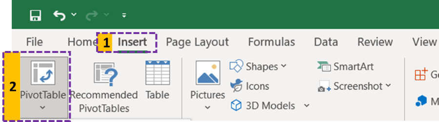
Img 1
Step 2: Enter your data set range in “Table/Range” input, choose New worksheet, and Click “OK
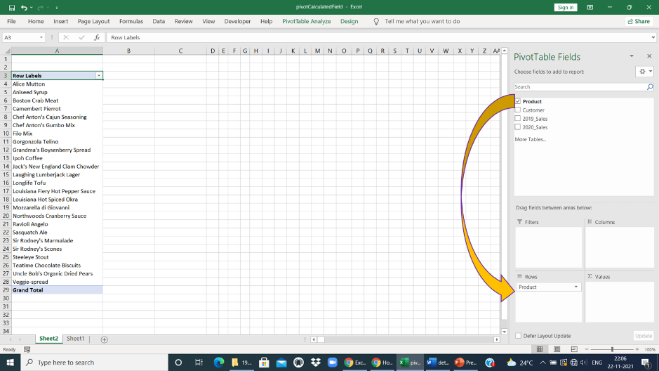
Step 3: Above step, add a new sheet with a pivot table for your data set.
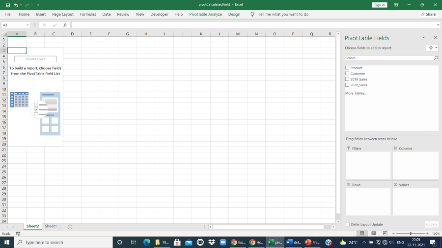
Pivot Table
Step 4: Drag the field “Products” to the Rows pane
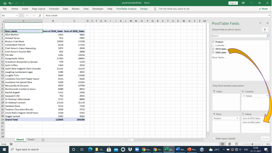
Step 5: Drag 2019_Sales and 2020_Sales to Values pane.
How to Add Calculated Field
You created a pivot table for your dataset. Now we add a calculated field to display the sales_differences in the pivot table
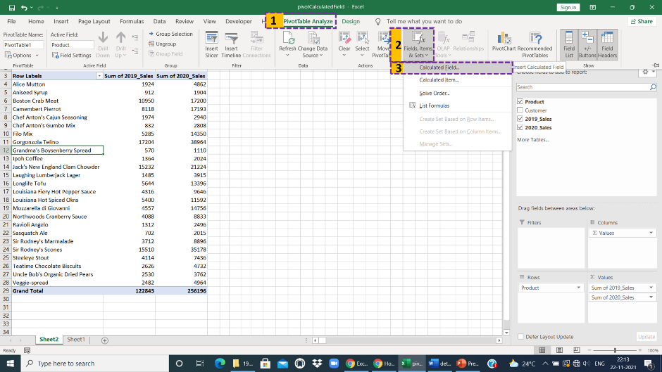
Step 6. To pop up the “Insert Calculated Field” dialogue box. Click anywhere in the pivot table. Goto PivotTable Analyze in Ribbon >> Fields, Items & Sets >> Calculated Field…
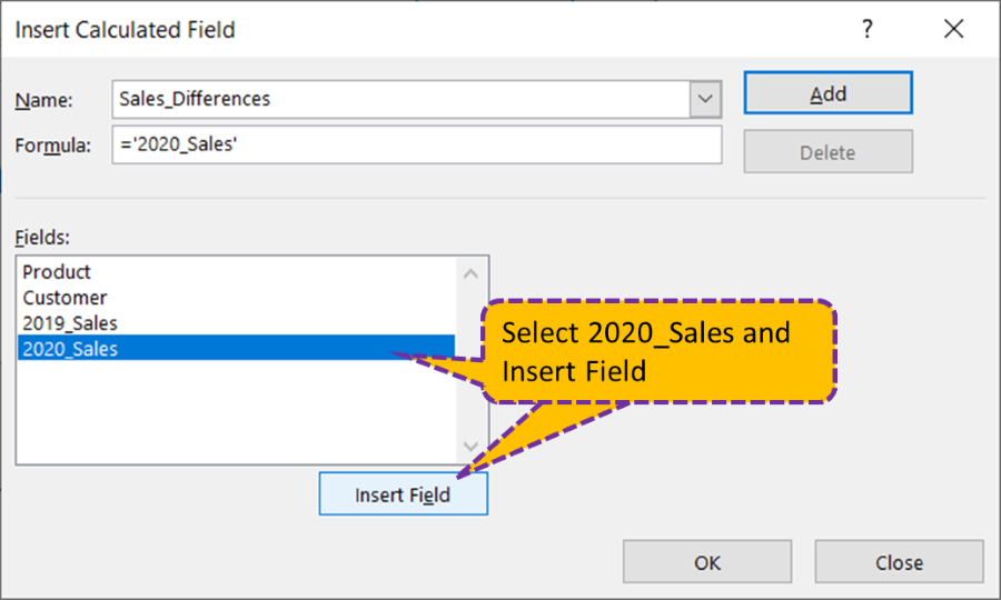
Step 7. Above step pop-up below dialogue box and type “Sales_Differences” [Calculated field Name] in the Name input box
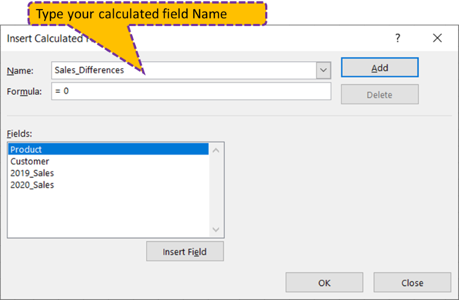
Step 8. Select “2020_Sales” from the fields list and Click Insert Field.
Step 9. Just type “-“ in Formula (for Subtraction).
Step 10. Select “2019_Sales” from the fields list and Click Insert Field.
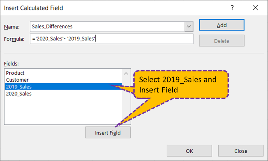
Step 11. Please make sure your formula is like below
='2020_Sales'-'2019_Sales'
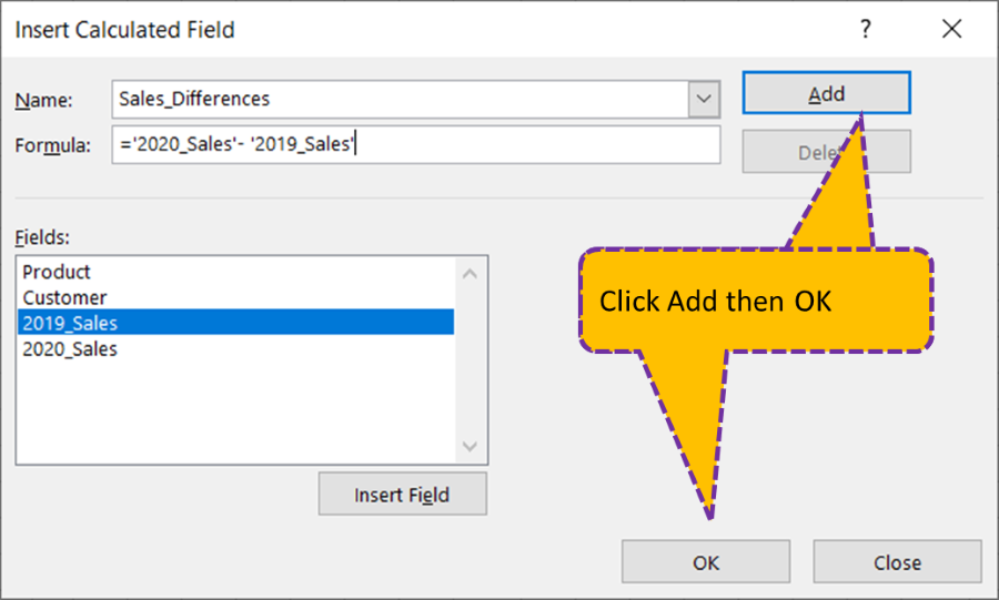
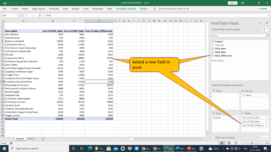
Step 12: Finally click Add then OK, you can see the pivot with additional columns “Sales_Differences” [Calculated Field] as in the below output
Output
About Calculated Fields
- For calculated fields, the sum of the individual values in the other value fields is used before doing the computation on the sum.
- All pivot tables based on the same pivot cache have calculated fields exposed by default.
What are Limitations of Calculated Fields
- Calculated field formulas cannot use the address or name of worksheet cells
- The pivot table totals or subtotals cannot be referenced in calculated field calculations
How to Modify or Delete a Pivot Table Calculated Field?
Following the procedures below, you can change or remove the formula in a Pivot Table Calculated Field:
Step 1. Select any cell in the Pivot Table
Step 2. Select Fields, Items, and Sets under Calculations from the Pivot Table Tools → Analyze

Analyze Tab
Step 3. Select Calculated Field
Step 4. Click on the drop-down arrow, In the Name field to select the calculated field you want to delete or modify
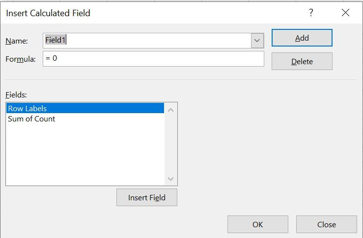
Insert Calculated Field

Modify or Delete Calculated Field
FAQs on Excel Pivot Table Calculated Field
1. What is the difference between calculated item and calculated field?
- Calculated Fields are formulas that can refer to other fields in the pivot table.
- Calculated Items are formulas that can make references to other items inside a certain pivot field.
Like Article
Suggest improvement
Share your thoughts in the comments
Please Login to comment...