Different Ways to Perform a Case-Sensitive Vlookup in Excel

In Excel datasets, sometimes you must have noticed, that there are many values in a table that are case-sensitive in nature. And if we want a particular type of value from our dataset, but unfortunately that value also has some duplicates, but with different case sensitivity, so here we need to search on the basis of case sensitivity. To make conditions worse, you only know one method to perform the search functions,i.e none other than VLOOKUP, and in nature, it is case-insensitive nature. What will you do? The only option to perform VLOOKUP in case of insensitivity is to optimize it using different methods.

But first, let us see how VLOOKUP is case-insensitive, by using an example:

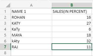
Now, let’s suppose we have this dataset of a company, and what we want, is how much “KaTy” has earned, and we only know the VLOOKUP function to perform it. So, applying VLOOKUP straightforward to find “KaTy” is not possible. Nonetheless, the output of applying VLOOKUP is going to be

VLOOKUP will look for approximation, rather than going for an exact match.VLOOKUP will look for the first encountered value and will return it. This is a problem, as first, we want an exact match to the keyword provided, and second of all, we want it to search the whole range provided. So, we will use some methods and functions to meet these conditions.

VLOOKUP CASE SENSITIVE FORMULA:

To do the above task using a formula, we can use VLOOKUP’s embedded formulas,i.e on what range you want to find values, the keyword, or the numeric value to be found, etc. So, the formula for doing the above task will be:

=VLOOKUP("KaTy",$A$2:$B$7,2)

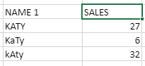
This will yield the same output table as obtained in the above example.It will search “KaTy” keyword in its default column,i.e column 1. The range for searching will be A2 to B7,i.e the whole dataset and the value for this keyword will be fetched from the 2nd column.

But, we want to make it case-sensitive by using some methods or some functions.

Here, we will use a virtual column,i.e known as a “Helper Column” in our formula, but technically, that column won’t be visible to us, as this helper function will be virtual in nature. Here, two functions, which are known as EXACT and CHOOSE are used. But first, let us apply the function and understand it part by part.

=VLOOKUP(MAX(EXACT("KaTy",$A$2:$A$7)*(ROW($A$2:$A$7))),CHOOSE({1,2},ROW($A$2:$A$7),$B$2:$B$7),2,0)

This will yield the following output:

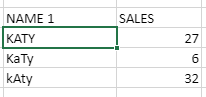
Now, these case-sensitive values, when called exclusively, will return separate values for each one of them, and not return 27 as redundant data every time. But, how did this formula worked? Let’s understand it part by part:

• EXACT(“KaTy”,$A$2:$A$7)–Exact always creates a boolean array, which will store true, whenever there is an exact carbon copy match of a given keyword in a given range, which in this case, is A2 TO A7.So, the array for this case will look like

{ FALSE;FALSE;TRUE;FALSE;FALSE;FALSE}

• (EXACT(“KaTy”,$A$2:$A$7)*(ROW($A$2:$A$7))–This method will multiply every boolean value of the above array, which was created by EXACT, and will multiply it with the row number of every cell from A2 TO A7. And, whenever the returned value is TRUE,it will put the row number of that entry in the same index, in the newly created array, and whenever the value is not matched, it will return 0. Keep in mind, that we are starting our range from A2,so row number 2 will be the initial searching row for us. Now, as row 4 contains “KaTy”, so the returned array will put number 4 in the 4th index of the newly created array. The array will look like this:

{0;0;4;0;0;0}

• (CHOOSE({1,2},ROW($A$2:$A$7),$B$2:$B$7)–Here the real magic is done by CHOOSE function only. This function will also create an array, but that array will look different from the above arrays. This function will basically register the row number from every cell encountered in the 1st range, which is A2 TO A7 and will assign their corresponding values from the 2nd range, which is B2 TO B7. Here,{1,2} will signify each element’s nature,i.e how the values will be stored in the array. Each element will have the row number and corresponding to it, its value. So, the array will look like

{2,16;3,27;4,6;5,18;6,32;7,11}

Here you can see, we are giving this unique identification to every argument of the dataset, and their case sensitivity is also undertaken here.

•  (MAX(EXACT(“KaTy”,$A$2:$A$7)*(ROW($A$2:$A$7)))– This will return the maximum value, or should we say the row number on which “KaTy” is stored in the dataset. So, if you look at the array which was returned by the EXACT function, the MAX value will be 4.

The VLOOKUP will look on the virtual array, or the helper dataset created by the CHOOSE function, and the MAX and EXACT will guide the VLOOKUP function.

SUMPRODUCT IN TEXT VALUES:

Now,if you have to lookup only at the numbers, and your return value is also number(s), so here we can use the SUMPRODUCT method. This method will help us multiply the values directly, by not using any helper column, and applying functions to it, hence saving our time. The declaration for this method will look like–

=SUMPRODUCT (--(1st array),array2*,array3*,...)

The arguments marked with asterick(*) are optional arrays(or columns), if not provided, it will find the sum of values of the first array. The “–” in this formula is only applied in the first array, and it will convert TRUE/FALSE values into 0/1 accordingly, as SUMPRODUCT works in numeric values arrays.

To understand the above syntax, we will see an example–

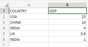
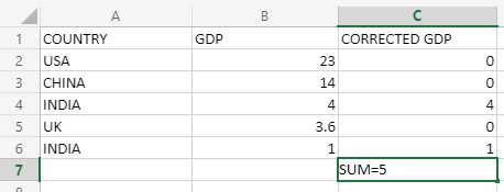
Here in this dataset, mistakenly INDIA’s GDP was written in two columns, and we have to return the total value of INDIA’S GDP.So, we will use SUMPRODUCT to do the task. First the formula will be:

=SUMPRODUCT(--(A2:A6="INDIA"),B2:B6)

When this formula is applied to C2 column, under the column name “CORRECTED GDP”,the returned dataset will be:

Now, how did this happen? What did SUMPRODUCT do? First of all, take a look at the representation of what happened in SUMPRODUCT’s implementation:

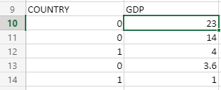
Here, as explained above, the “–” converted the returned value of the “=” function, which was either TRUE or FALSE, and it converted TRUE into 1, and FALSE into 0. Then sumproduct did a multiplication function on these two arrays(columns), and the above representation shows, how it is done.

We were searching for the keyword “INDIA” in A2 TO A6, and after conversion by the “–“(double negation), the corresponding values are multiplied, and the result is stored in other columns, named as CORRECTED GDP.So, the corrected GDP for INDIA is 5 trillion$.

INDEX MATCH, a LOOKUP method for case-sensitive searching:

INDEX MATCH is probably the best contender for doing case-sensitive lookups in Excel. But, why? There are some points, that make INDEX MATCH lookup method very preferable in the lookup areas-

1. Whatever data type you have, that has to look up, whether it is file, text, numerics, alphanumerics, etc,it is compatible on almost any data type you want.
2. If you know the basics of the LOOKUP method, you must know that this method requires you to sort the lookup column, but in INDEX MATCH, there is no problem like this,i.e it works on unsorted lookup columns too.
3. It does not require any helper column too.

Here, the MATCH function or INDEX function alone can’t achieve case-sensitive lookups, so we will use a method known as EXACT. As EXACT was helping VLOOKUP to achieve case sensitivity, here EXACT, combined with MATCH and INDEX function will make the INDEX MATCH method case-sensitive.

The syntax for this method will be:

{=INDEX(data from which value will be fetched by searching,MATCH(TRUE/FALSE,EXACT(Lookup Column Range,key),0))}

Note: As this formula is treated as an array function, so we will use Ctrl+Shift+Enter to execute the formula.

Now, we will understand the working and the syntax of this formula through an example–

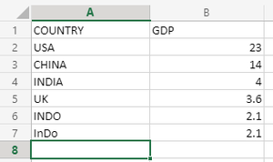
Now, here in this dataset, the data entry person made a mistake and entered INDONESIA’s GDP two times in the same dataset, and we know is that the one with the “INDO” keyword is the correct one, and we will fetch its GDP. Now, we will use INDEX MATCH to accomplish it. The formula for this will be:

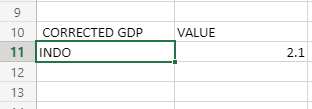
{=INDEX($B$2:$B$7,MATCH(TRUE,EXACT($A$2:$A$7,"INDO"),0))}

This will output us the GDP of “INDO”,i.e Indonesia, which is 2.1.

Now, we will understand its working part by part:

1. EXACT($A$2:$A$7,”INDO”)–This will search for the keyword “INDO” in the given range, ie from A2 to A7, and the match will be exact.
2. MATCH(TRUE,EXACT($A$2:$A$7,”INDO”)–This will return us the row number, on which the given keyword has been matched exactly, which in this case is 5.
3. INDEX($B$2:$B$7,MATCH(TRUE,EXACT($A$2:$A$7,”INDO”),0))–This will search for the value in the given range, on which the given keyword in the range A2 to A7 has been matched, ie it will return 2.1 to us.