Denoising techniques in digital image processing using MATLAB
Last Updated :
28 Dec, 2022
Denoising is the process of removing or reducing the noise or artifacts from the image. Denoising makes the image more clear and enables us to see finer details in the image clearly. It does not change the brightness or contrast of the image directly, but due to the removal of artifacts, the final image may look brighter.
In this denoising process, we choose a 2-D box and slide it over the image. The intensity of each and every pixel of the original image is recalculated using the box.
Box averaging technique:
Box averaging can be defined as the intensity of the corresponding pixel would be replaced with the average of all intensities of its neighbour pixels spanned by the box. This is a point operator.
Now, let’s suppose the box size is 5 by 5. It will span over 25 pixels at one time. The intensity value of the central pixel (point operator on central pixel) will be the average of intensities of all the 25 pixels covered by the box of 5 by 5 dimensions.
Example:
Matlab
k1=imread("cameraman.jpg");
n=25*randn(size(k1));
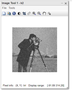
k2=double(k1)+n;
imtool(k2,[]);
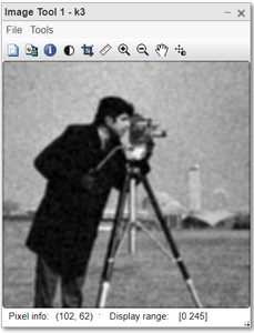
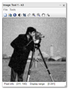
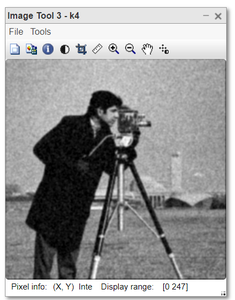
k3=uint8(colfilt(k2,[5 5], 'sliding', @mean));
imtool(k3,[]);
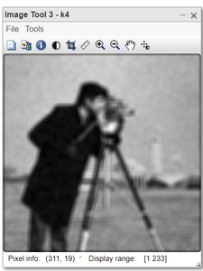
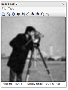
k4=uint8(colfilt(k2, [9 9], 'sliding', @mean));
imtool(k4,[]);
|
Output:
But there are some disadvantages of this technique:
- It reduces the noise to a small extent but introduces blurriness in the image.
- If we increase the box size then smoothness and blurriness in the image increase proportionately.
Simple and gaussian convolution techniques:
Convolution does a similar work as the box averaging. In the convolution technique, we define the box and initialise it with the values. For denoising purposes, we initialise the box such that it behaves like averaging box. The convolution box is called the kernel. The kernel slides over the image. The value of the central pixel is replaced by the average of all the neighbour pixels spanned by the kernel.
kernel working: The values of the kernel and respective pixel got multiplied and all such products got added to give the final result. If our kernel is of size [5 5] then we initialise the kernel with 1/25. When all the pixels got multiplied by 1/25 and added together, the final result is just the average of all those 25 pixels over which the kernel is placed at a certain point in time.
The advantage of convolution over box averaging is that sometimes the convolution filter (kernel) is separable and we break the larger kernel into two or more pieces. It reduces the computational operations to perform.
Example:
Matlab
k1=imread("cameraman.jpg");
n=25*randn(size(k1));
k2=double(k1)+n;
h1=ones(5,5)*1/25;
k3=uint8(conv2(k2, h1,'same'));
imtool(k3,[]);
h2=ones(9,9)*1/81;
k4=conv2(k2,h2,'same');
imtool(k4,[]);
|
Output:
A drawback of this technique is:
- It also introduces the blurriness in the image in addition to reducing the noise.
- The image gets blurred at the edges due to the wrong averaging result.
Gaussian Filter:
This kernel or filter has more weightage for the central pixel. While averaging at the edges, more weightage is given to the edged pixel and thus it gives us the pixel value close to the actual one, therefore, reduces the blurriness at the edges.
Keep in mind that if we increase the size of the filter, the degree of denoising increases and also the blurriness. But blurriness is significantly less in comparison to other averaging techniques.
Example:
Matlab
k1=imread("cameraman.jpg");
n=25*randn(size(k1));
k2=double(k1)+n;
h1=fspecial('gaussian',3,1);
h1
k3=uint8(conv2(k2, h1,'same'));
imtool(k3,[]);
h2=fspecial('gaussian',20,1);
h2
k4=uint8(conv2(k2,h2,'same'));
imtool(k4,[]);
|
Output:

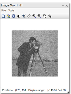
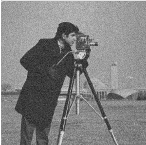
Denoising by averaging noisy images:
This is a very simple and interesting technique of denoising. The requirement for using this technique is that:
- We should have 2 or more images of the same scene or object.
- The noise of the image capturing device should be fixed. For example, the camera has a noise of a standard deviation of 20.
Working:
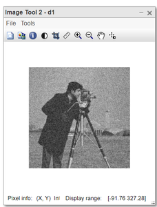
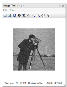
Collect the multiple images captured by the same device and of the same object. Just take the average of all the images to get the resultant image. The intensity of every pixel will be replaced by the average of the intensities of the corresponding pixel in all those collected images.This technique will reduce the noise and also there would not be any blurriness in the final image.
Let say we have n images. Then the noise will be reduced by the degree: 
The more number images used for averaging the more clear image we’ll get after denoising.
Example:
Matlab
I=imread("cameraman.jpg");
n1=40*randn(size(I));
I1=double(I)+n1;
n2=40*randn(size(I));
I2=double(I)+n2;
n3=40*randn(size(I));
I3=double(I)+n3;
n4=40*randn(size(I));
I4=double(I)+n4;
n5=40*randn(size(I));
I5=double(I)+n5;
d1=(I1+I2)/2;
d2=(I1+I2+I3)/3;
d3=(I1+I2+I3+I4)/4;
d4=(I1+I2+I3+I4+I5)/5;
imtool(I1,[]);
imtool(d1,[]);
imtool(d2,[]);
imtool(d3,[]);
imtool(d4,[]);
|
Output:
Noisy_image and Denoised-1
Noisy_image and Denoised-2
Noisy_image and Denoised-3
Noisy_image and Denoised-4
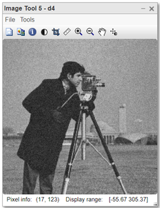
The quality increases directly if we take more images for averaging.
Like Article
Suggest improvement
Share your thoughts in the comments
Please Login to comment...