Deep Learning Interview Questions

Deep learning is a part of machine learning that is based on the artificial neural network with multiple layers to learn from and make predictions on data. An artificial neural network is based on the structure and working of the Biological neuron which is found in the brain.

Deep Learning Interview Questions 2023

This Deep Learning Interview Questions and answers cover all the basic to advanced Interview questions on Deep learning which will give you the confidence to stand in a tech interview. These Deep Learning Interview Questions are suggested questions by highly experienced data scientist professionals. So, this will definitely give you an edge in your Deep Learning Interview.

• Deep Learning Interview Questions for Freshers
• Deep Learning Interview Questions for Experienced

Deep Learning Interview Questions For Freshers

1. What is Deep Learning?

Deep learning is the branch of machine learning which is based on artificial neural network architecture which makes it capable of learning complex patterns and relationships within data. An artificial neural network or ANN uses layers of interconnected nodes called neurons that work togeather to process and learn from the input data.

In a fully connected Deep neural network, there is an input layer and one or more hidden layers connected one after the other. Each neuron receives input from the previous layer neurons or the input layer. The output of one neuron becomes the input to other neurons in the next layer of the network, and this process continues until the final layer produces the output of the network. The layers of the neural network transform the input data through a series of nonlinear transformations, allowing the network to learn complex representations of the input data.

 Today Deep learning has become one of the most popular and visible areas of machine learning, due to its success in a variety of applications, such as computer vision, natural language processing, and Reinforcement learning.

2. What is an artificial neural network?

An artificial neural network is inspired by the networks and functionalities of human biological neurons. it is also known as neural networks or neural nets. ANN uses layers of interconnected nodes called artificial neurons that work together to process and learn the input data. The starting layer artificial neural network is known as the input layer, it takes input from external input sources and transfers it to the next layer known as the hidden layer where each neuron received inputs from previous layer neurons and computes the weighted sum, and transfers to the next layer neurons. These connections are weighted means effects of the inputs from the previous layer are optimized more or less by assigning different-different weights to each input and it is adjusted during the training process by optimizing these weights for better performance of the model. The output of one neuron becomes the input to other neurons in the next layer of the network, and this process continues until the final layer produces the output of the network.

artificial neural network

3. How does Deep Learning differ from Machine Learning?

Machine learning and deep learning both are subsets of artificial intelligence but there are many similarities and differences between them.

Machine Learning	Deep Learning
Apply statistical algorithms to learn the hidden patterns and relationships in the dataset.	Uses artificial neural network architecture to learn the hidden patterns and relationships in the dataset.
Can work on the smaller amount of dataset	Requires the larger volume of dataset compared to machine learning
Better for the low-label task.	Better for complex tasks like image processing, natural language processing, etc.
Takes less time to train the model.	Takes more time ta o train the model.
A model is created by relevant features which are manually extracted from images to detect an object in the image.	Relevant features are automatically extracted from images. It is an end-to-end learning process.
Less complex and easy to interpret the result.	More complex, it works like the black box interpretations of the result are not easy.
It can work on the CPU or requires less computing power as compared to deep learning.	It requires a high-performance computer with GPU.

4. What are the applications of Deep Learning?

Deep learning has many applications, and it can be broadly divided into computer vision, natural language processing (NLP), and reinforcement learning. 

• Computer vision:  Deep learning employs neural networks with several layers, which enables it used for automated learning and recognition of complex patterns in images. and machines can perform image classification, image segmentation, object detection, and image generation task accurately. It has greatly increased the precision and effectiveness of computer vision algorithms, enabling a variety of uses in industries including healthcare, transportation, and entertainment.
• Natural language processing (NLP): Natural language processing (NLP) gained enormously from deep learning, which has enhanced language modeling, sentiment analysis, and machine translation. Deep learning models have the ability to automatically discover complex linguistic features from text data, enabling more precise and effective processing of inputs in natural language.
• Reinforcement learning: Deep learning is used in reinforcement learning to evaluate the value of various actions in various states, allowing the agent to make better decisions that can maximize the predicted rewards. By learning from these mistakes, an agent eventually raises its performance. Deep learning applications that use reinforcement learning include gaming, robotics, and control systems.

5. What are the challenges in Deep Learning?

Deep learning has made significant advancements in various fields, but there are still some challenges that need to be addressed. Here are some of the main challenges in deep learning:

1. Data availability: It requires large amounts of data to learn from. For using deep learning it’s a big concern to gather as much data for training.
2. Computational Resources: For training the deep learning model, it is computationally expensive because it requires specialized hardware like GPUs and TPUs.
3. Time-consuming: While working on sequential data depending on the computational resource it can take very large even in days or months. 
4. Interpretability: Deep learning models are complex, it works like a black box. it is very difficult to interpret the result.
5. Overfitting: when the model is trained again and again, it becomes too specialized for the training data, leading to overfitting and poor performance on new data.

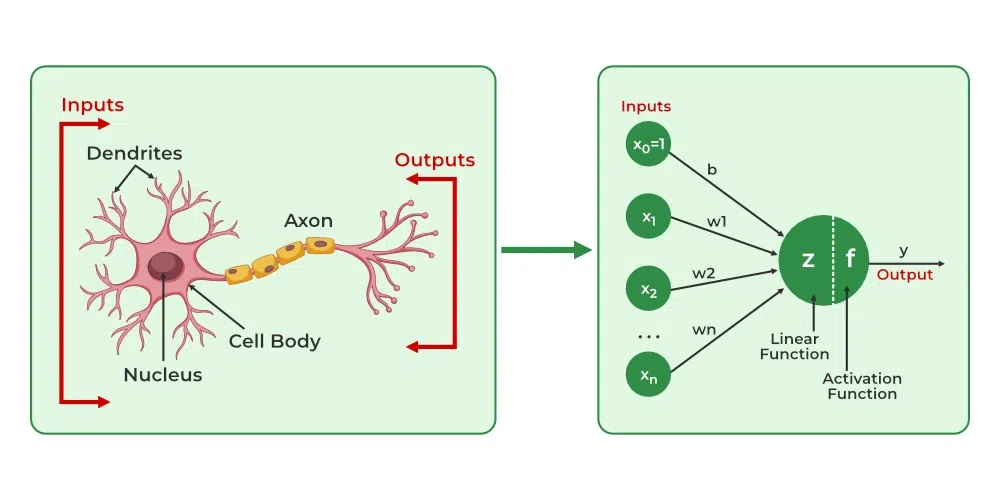
6. How Biological neurons are similar to the Artificial neural network.

The concept of artificial neural networks comes from biological neurons found in animal brains So they share a lot of similarities in structure and function wise.

• Structure: The structure of artificial neural networks is inspired by biological neurons. A biological neuron has dendrites to receive the signals, a cell body or soma to process them, and an axon to transmit the signal to other neurons.  In artificial neural networks input signals are received by input nodes, hidden layer nodes compute these input signals, and output layer nodes compute the final output by processing the outputs of the hidden layer using activation functions.
• Synapses: In biological neurons, synapses are the connections between neurons that allow for the transmission of signals from dendrites to the cell body and the cell body to the axon like that. In artificial neurons, synapses are termed as the weights which connect the one-layer nodes to the next-layer nodes. The weight value determines the strength between the connections. 
• Learning: In biological neurons, learning occurs in the cell body or soma which has a nucleus that helps to process the signals. If the signals are strong enough to reach the threshold, an action potential is generated that travels through the axons. This is achieved by synaptic plasticity, which is the ability of synapses to strengthen or weaken over time, in response to increases or decreases in their activity. In artificial neural networks, the learning process is called backpropagations, which adjusts the weight between the nodes based on the difference or cost between the predicted and actual outputs.
• Activation: In biological neurons, activation is the firing rate of the neuron which happens when the signals are strong enough to reach the threshold. and in artificial neural networks, activations are done by mathematical functions known as activations functions which map the input to the output.

Biological neurons to Artificial neurons

7. How deep learning is used in supervised, unsupervised as well as reinforcement machine learning?

Deep learning can be used for supervised, unsupervised as well as reinforcement machine learning. it uses a variety of ways to process these.

• Supervised Machine Learning: Supervised machine learning is the machine learning technique in which the neural network learns to make predictions or classify data based on the labeled datasets. Here we input both input features along with the target variables. the neural network learns to make predictions based on the cost or error that comes from the difference between the predicted and the actual target, this process is known as backpropagation.  Deep learning algorithms like Convolutional neural networks, Recurrent neural networks are used for many supervised tasks like image classifications and recognization, sentiment analysis, language translations, etc.
• Unsupervised Machine Learning: Unsupervised machine learning is the machine learning technique in which the neural network learns to discover the patterns or to cluster the dataset based on unlabeled datasets. Here there are no target variables. while the machine has to self-determined the hidden patterns or relationships within the datasets. Deep learning algorithms like autoencoders and generative models are used for unsupervised tasks like clustering, dimensionality reduction, and anomaly detection.
• Reinforcement  Machine Learning: Reinforcement  Machine Learning is the machine learning technique in which an agent learns to make decisions in an environment to maximize a reward signal. The agent interacts with the environment by taking action and observing the resulting rewards. Deep learning can be used to learn policies, or a set of actions, that maximizes the cumulative reward over time. Deep reinforcement learning algorithms like Deep Q networks and Deep Deterministic Policy Gradient (DDPG) are used to reinforce tasks like robotics and game playing etc.

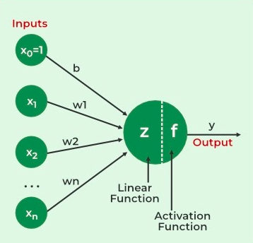
8. What is a Perceptron?

Perceptron is one of the simplest Artificial neural network architectures. It was introduced by Frank Rosenblatt in 1957s. It is the simplest type of feedforward neural network, consisting of a single layer of input nodes that are fully connected to a layer of output nodes. It can learn the linearly separable patterns. it uses slightly different types of artificial neurons known as threshold logic units (TLU). it was first introduced by McCulloch and Walter Pitts in the 1940s. it computes the weighted sum of its inputs and then applies the step function to compare this weighted sum to the threshold. the most common step function used in perceptron is the Heaviside step function.

A perceptron has a single layer of threshold logic units with each TLU connected to all inputs. When all the neurons in a layer are connected to every neuron of the previous layer, it is known as a fully connected layer or dense layer. During training, The weights of the perceptron are adjusted to minimize the difference between the actual and predicted value using the perceptron learning rule i.e 

w_i = w_i + (learning_rate * (true_output - predicted_output) * x_i)

Here, x_i and w_i are the i^th input feature and the weight of the i^th input feature.

9.  What is Multilayer Perceptron? and How it is different from a single-layer perceptron?

A multilayer perceptron (MLP) is an advancement of the single-layer perceptron which uses more than one hidden layer to process the data from input to the final prediction. It consists of multiple layers of interconnected neurons, with multiple nodes present in each layer. The MLP architecture is referred to as the feedforward neural network because data flows in one direction, from the input layer through one or more hidden layers to the output layer.  

The differences between the single-layer perceptron and multilayer perceptron are as follows:

• Architecture: A single-layer perceptron has only one layer of neurons, which takes the input and produces an output. While a multilayer perceptron has one or more hidden layers of neurons between the input and output layers. 
• Complexity: A single-layer perceptron is a simple linear classifier that can only learn linearly separable patterns. While a multilayer perceptron can learn more complex and nonlinear patterns by using nonlinear activation functions in the hidden layers. 
• Learning: Single-layer perceptrons use a simple perceptron learning rule to update their weights during training. While multilayer perceptrons use a more complex backpropagation algorithm to train their weights, which involves both forward propagations of input through the network and backpropagation of errors to update the weights. 
• Output: Single-layer perceptrons produce a binary output, indicating which of two possible classes the input belongs to. Multilayer perceptrons can produce real-valued outputs, allowing them to perform regression tasks in addition to classification.
• Applications: Single-layer perceptrons are suitable for simple linear classification tasks whereas Multilayer perceptrons are more suitable for complex classification tasks where the input data is not linearly separable, as well as for regression tasks where the output is continuous variables.

10. What are Feedforward Neural Networks?

A feedforward neural network (FNN) is a type of artificial neural network, in which the neurons are arranged in layers, and the information flows only in one direction, from the input layer to the output layer, without any feedback connections. The term “feedforward” means information flows forward through the neural network in a single direction from the input layer through one or more hidden layers to the output layer without any loops or cycles.

In a feedforward neural network (FNN) the weight is updated after the forward pass. During the forward pass, the input is fed and it computes the prediction after the series of nonlinear transformations to the input. then it is compared with the actual output and errors are calculated.

During the backward pass also known as backpropagation, Based on the differences, the error is first propagated back to the output layer, where the gradient of the loss function with respect to the output is computed. This gradient is then propagated backward through the network to compute the gradient of the loss function with respect to the weights and biases of each layer. Here chain rules of calculus are applied with respect to weight and bias to find the gradient. These gradients are then used to update the weights and biases of the network so that it can improve its performance on the given task. 

11. What is GPU?

A graphics processing unit, sometimes known as a GPU, is a specialized electronic circuit designed to render graphics and images on a computer or other digital device fast and effectively.

Originally developed for use in video games and other graphical applications, GPUs have grown in significance in a number of disciplines, such as artificial intelligence, machine learning, and scientific research, where they are used to speed up computationally demanding tasks like training deep neural networks.

One of the main benefits of GPUs is their capacity for parallel computation, which uses a significant number of processing cores to speed up complicated calculations. Since high-dimensional data manipulations and matrix operations are frequently used in machine learning and other data-driven applications, these activities are particularly well suited for them.

12. What are the different layers in ANN? What is the notation for representing a node of a particular layer?

There are commonly three different types of layers in an artificial neural network (ANN):

• Input Layer: This is the layer that receives the input data and passes it on to the next layer. The input layer is typically not counted as one of the hidden layers of the network. 
• Hidden Layers: The input layer is the one that receives input data and transfers it to the next layer. Usually, the input layer is not included in the list of the hidden layers of the neural network. 
• Output Layer: This is the output-producing layer of the network. A binary classification problem might only have one output neuron, but a multi-class classification problem might have numerous output neurons, one for each class. The number of neurons in the output layer depends on the type of problem being solved. 

We commonly use a notation like  to represent a node of a specific layer in an ANN, where L denotes the layer number and i denotes the node’s index inside that layer. For instance, the input layer’s first node may be written as  whereas the third hidden layer’s second node might be written as  With this notation, it is simple to refer to specific network nodes to understand the structure of the network as a whole.

13. What is forward and backward propagation?

In deep learning and neural networks, In the forward pass or propagation, The input data propagates through the input layer to the hidden layer to the output layer. During this process, each layer of the neural network performs a series of mathematical operations on the input data and transfers it to the next layer until the output is generated.

Once the forward propagation is complete, the backward propagation, also known as backpropagation or back prop, is started. During the backward pass, the generated output is compared to the actual output and based on the differences between them the error is measured and it is propagated backward through the neural network layer. Where the gradient of the loss function with respect to the output is computed. This gradient is then propagated backward through the network to compute the gradient of the loss function with respect to the weights and biases of each layer. Here chain rules of calculus are applied with respect to weight and bias to find the gradient. These gradients are then used to update the weights and biases of the network so that it can improve its performance on the given task. 

 In simple terms, the forward pass involves feeding input data into the neural network to produce an output,  while the backward pass refers to utilizing the output to compute the error and modify the network’s weights and biases.

14. What is the cost function in deep learning?

The cost function is the mathematical function that is used to measure the quality of prediction during training in deep neural networks. It measures the differences between the generated output of the forward pass of the neural network to the actual outputs, which are known as losses or errors. During the training process, the weights of the network are adjusted to minimize the losses. which is achieved by computing the gradient of the cost function with respect to weights and biases using backpropagation algorithms.

 The cost function is also known as the loss function or objective function. In deep learning, different -different types of cost functions are used depending on the type of problem and neural network used.  Some of the common cost functions are as follows:

• Binary Cross-Entropy for binary classification measures the difference between the predicted probability of the positive outcome and the actual outcome.
• Categorical Cross-Entropy for multi-class classification measures the difference between the predicted probability and the actual probability distribution.
• Sparse Categorical Cross-Entropy for multi-class classification is used when the actual label is an integer rather than in a one-hot encoded vector.
• Kullback-Leibler Divergence (KL Divergence) is used in generative learning like Generative Adversarial Networks (GANs) and Variational Autoencoders (VAEs), it measures the differences between two probability distributions.
• Mean Squared Error for regression to measure the average squared difference between actual and predicted outputs.

15. What are activation functions in deep learning and where it is used?

Deep learning uses activation functions, which are mathematical operations that are performed on each neuron’s output in a neural network to provide nonlinearity to the network. The goal of activation functions is to inject non-linearity into the network so that it can learn the more complex relationships between the input and output variables. 

In other words, the activation function in neural networks takes the output of the preceding linear operation (which is usually the weighted sum of input values i.e w*x+b) and mapped it to a desired range because the repeated application of weighted sum (i.e w*x +b) will result in a polynomial function. The activation function transformed the linear output into non-linear output which makes the neural network capable to approximate more complex tasks.

In deep learning, To compute the gradients of the loss function with respect to the network weights during backpropagation, activation functions must be differentiable. As a result, the network may use gradient descent or other optimization techniques to find the optimal weights to minimize the loss function.

Although several activation functions, such as ReLU, and Hardtanh, contain point discontinuities, they are still differentiable almost everywhere. The gradient is not defined at the point of discontinuity, This does not have a substantial impact on the network’s overall gradient because the gradient at these points is normally set to zero or a small value.

16. What are the different different types of activation functions used in deep learning?

In deep learning, several different-different types of activation functions are used. Each of them has its own strength and weakness. Some of the most common activation functions are as follows.

• Sigmoid function: It maps any value between 0 and 1. It is mainly used in binary classification problems. where it maps the output of the preceding hidden layer into the probability value.
• Softmax function: It is the extension of the sigmoid function used for multi-class classification problems in the output layer of the neural network, where it maps the output of the previous layer into a probability distribution across the classes, giving each class a probability value between 0 and 1 with the sum of the probabilities over all classes is equal to 1. The class which has the highest probability value is considered as the predicted class.
• ReLU (Rectified Linear Unit) function: It is a non-linear function that returns the input value for positive inputs and 0 for negative inputs. Deep neural networks frequently employ this function since it is both straightforward and effective.
• Leaky ReLU function: It is similar to the ReLU function, but it adds a small slope for negative input values to prevent dead neurons.
• Tanh (hyperbolic tangent) function: It is a non-linear activations function that maps the input’s value between -1 to 1. It is similar to the sigmoid function but it provides both positive and negative results. It is mainly used for regression tasks, where the output will be continuous values.

17. How do neural networks learn from the data?

In neural networks, there is a method known as backpropagation is used while training the neural network for adjusting weights and biases of the neural network. It computes the gradient of the cost functions with respect to the parameters of the neural network and then updates the network parameters in the opposite direction of the gradient using optimization algorithms with the aim of minimizing the losses.

During the training, in forward pass the input data passes through the network and generates output. then the cost function compares this generated output to the actual output. then the backpropagation computes the gradient of the cost function with respect to the output of the neural network. This gradient is then propagated backward through the network to compute the gradient of the loss function with respect to the weights and biases of each layer. Here chain rules of differentiations are applied with respect to the parameters of each layer to find the gradient. 

Once the gradient is computed, The optimization algorithms are used to update the parameters of the network. Some of the most common optimization algorithms are stochastic gradient descent (SGD), mini-batch, etc.

The goal of the training process is to minimize the cost function by adjusting the weights and biases during the backpropagation.

18. How the number of hidden layers and number of neurons per hidden layer are selected?

There is no one-size-fits-all solution to this problem, hence choosing the number of hidden layers and neurons per hidden layer in a neural network is often dependent on practical observations and experimentation. There are, however, a few general principles and heuristics that may be applied as a base.

• The number of hidden layers can be determined by the complexity of the problem being solved. Simple problems can be solved with just one hidden layer whereas more complicated problems may require two or more hidden levels. However adding more layers also increases the risk of overfitting, so the number of layers should be chosen based on the trade-off between model complexity and generalization performance.
• The number of neurons per hidden layer can be determined based on the number of input features and the desired level of model complexity. There is no hard and fast rule, and the number of neurons can be adjusted based on the results of experimentation and validation.

In practice, it is often useful to start with a simple model and gradually increase its complexity until the desired performance is achieved. This process can involve adding more hidden layers or neurons or experimenting with different architectures and hyperparameters. It is also important to regularly monitor the training and validation performance to detect overfitting and adjust the model accordingly.

19. What is overfitting and how to avoid it?

Overfitting is a problem in machine learning that occurs when the model learns to fit the training data too close to the point that it starts catching up on noise and unimportant patterns. Because of this, the model performs well on training data but badly on fresh, untested data, resulting in poor generalization performance.

To avoid overfitting in deep learning we can use the following techniques:

1. Simplify the model: Overfitting may be less likely in a simpler model with fewer layers and parameters. In practical applications, it is frequently beneficial, to begin with a simple model and progressively increase its complexity until the desired performance is attained.
2. Regularization: Regularization is a technique used in machine learning to prevent the overfitting of a model by adding a penalty term, it imposes the constraint on the weight of the model. Some of the most common regularization techniques are as follows:
   1. L1 and L2 regularization: L1 regularization sparse the model by equating many model weights equal to 0 while L2 regularization constrains the weight of the neural network connection.
   2. Dropout: Dropout is a technique that randomly drops out or disables some of the randomly selected neurons. It is applied after the activation functions of the hidden layer. Typically, it is set to a small value like 0.2 or 0.25. For the dropout value of 0.20, Each neuron in the previously hidden layer has a 20% chance of being inactive. It is only operational during the training process.
   3. Max-Norm Regularization: It constrains the magnitude of the weights in a neural network by setting a maximum limit (or norm) on the weights of the neurons, such that their values cannot exceed this limit.
3. Data augmentation: By applying various transformations, such as rotating or flipping images, to new training data, it is possible to teach the model to become more robust to changes in the input data.
4. Increasing the amount of training data: By increasing the amount of data can provide the model with a diverse set of examples to learn from, which can be helpful to prevent overfitting.
5. Early stopping: This involves keeping track of the model’s performance on a validation set during training and terminating the training process when the validation loss stops decreasing.

20. Define epoch, iterations, and batches.

A complete cycle of deep learning model training utilizing the entire training dataset is called an epoch. Each training sample in the dataset is processed by the model during a single epoch, and its weights and biases are adjusted in response to the estimated loss or error. The number of epochs will range from 1 to infinite. User input determines it. It is always an Integral value.

Iteration refers to the procedure of running a batch of data through the model, figuring out the loss, and changing the model’s parameters. Depending on the number of batches in the dataset, one or more iterations can be possible within a single epoch.

A batch in deep learning is a subset of the training data that is used to modify the weights of a model during training. In batch training, the entire training set is divided into smaller groups, and the model is updated after analyzing each batch.  An epoch can be made up of one or more batches.

• The batch size will be more than one and always less than the number of samples.
• Batch size is a hyperparameter, it is set by the user. where the number of iterations per epoch is calculated by dividing the total number of training samples by the individual batch size.

Deep learning training datasets are often separated into smaller batches, and the model analyses each batch sequentially, one at a time, throughout each epoch.  On the validation dataset, the model performance can be assessed after each epoch. This helps in monitoring the model’s progress. 

For example: Let’s use 5000 training samples in the training dataset. Furthermore, we want to divide the dataset into 100 batches. If we choose to use five epochs, the total number of iterations will be as follows:

Total number of training samples = 5000
Batch size = 100
Total number of iterations=Total number of training samples/Batch size=5000/100=50
Total number of iterations = 50
One epoch = 50 iterations
Total number of iterations in 5 epochs = 50*5 = 250 iterations.

21. Define the learning rate in Deep Learning.

The learning rate in deep learning is a hyperparameter that controls how frequently the optimizer adjusts the neural network’s weights when it is being trained. It determines the step size to which the optimizer frequently updates the model parameters with respect to the loss function. so, that losses can be minimized during training.

With the high learning rate, the model may converge fast, but it may also overshoot or bounce around the ideal solution. On the other hand, a low learning rate might make the model converge slowly, but it could also produce a solution that is more accurate.

Choosing the appropriate learning rate is crucial for the successful training of deep neural networks.

22. What is the cross-entropy loss function?

Cross-entropy is the commonly used loss function in deep learning for classification problems. The cross-entropy loss measures the difference between the real probability distribution and the predicted probability distribution over the classes.

The formula for the Cross-Entropy loss function for the K classes will be:

Here, Y and  are actual and predicted values for a single instance. k represents a particular class and is a subset of K.

23. What is gradient descent?

Gradient descent is the core of the learning process in machine learning and deep learning. It is the method used to minimize the cost or loss function by iteratively adjusting the model parameters i.e. weight and biases of the neural layer. The objective is to reduce this disparity, which is represented by the cost function as the difference between the model’s anticipated output and the actual output.

The gradient is the vector of its partial derivatives with respect to its inputs, which indicates the direction of the steepest ascent (positive gradient) or steepest descent (negative gradient) of the function. 

In deep learning, The gradient is the partial derivative of the objective or cost function with respect to its model parameters i.e. weights or biases, and this gradient is used to update the model’s parameters in the direction of the negative gradient so that it can reduce the cost function and increase the performance of the model. The magnitude of the update is determined by the learning rate, which controls the step size of the update.

24. How do you optimize a Deep Learning model?

A Deep Learning model may be optimized by changing its parameters and hyperparameters to increase its performance on a particular task. Here are a few typical methods for deep learning model optimization:

• Choosing the right architecture
• Adjusting the learning rate
• Regularization
• Data augmentation
• Transfer learning
• Hyperparameter tuning

25. Define Batch, Stochastic, and Mini gradient descent.

There are several variants of gradient descent that differ in the way the step size or learning rate is chosen and the way the updates are made. Here are some popular variants:

• Batch Gradient Descent: In batch gradient descent, To update the model parameters values like weight and bias, the entire training dataset is used to compute the gradient and update the parameters at each iteration. This can be slow for large datasets but may lead to a more accurate model. It is effective for convex or relatively smooth error manifolds because it moves directly toward an optimal solution by taking a large step in the direction of the negative gradient of the cost function. However, it can be slow for large datasets because it computes the gradient and updates the parameters using the entire training dataset at each iteration. This can result in longer training times and higher computational costs.
• Stochastic Gradient Descent (SGD): In SGD, only one training example is used to compute the gradient and update the parameters at each iteration. This can be faster than batch gradient descent but may lead to more noise in the updates.
• Mini-batch Gradient Descent: In Mini-batch gradient descent a small batch of training examples is used to compute the gradient and update the parameters at each iteration. This can be a good compromise between batch gradient descent and Stochastic Gradient Descent, as it can be faster than batch gradient descent and less noisy than Stochastic Gradient Descent.

26. What are the different types of Neural Networks?

There are different-different types of neural networks used in deep learning. Some of the most important neural network architectures are as follows;

1. Feedforward Neural Networks (FFNNs)
2. Convolutional Neural Networks (CNNs)
3. Recurrent Neural Networks (RNNs)
4. Long Short-Term Memory Networks (LSTMs)
5. Gated Recurrent Units (GRU)
6. Autoencoder Neural Networks
7. Attention Mechanism
8. Generative Adversarial Networks (GANs)
9. Transformers
10. Deep Belief Networks (DBNs)

27. What is the difference between Shallow Networks and Deep Networks?

Deep networks and shallow networks are two types of artificial neural networks that can learn from data and perform tasks such as classification, regression, clustering, and generation.

• Shallow networks: A shallow network has a single hidden layer between the input and output layers, whereas a deep network has several hidden layers. Because they have fewer parameters, they are easier to train and less computationally expensive than deep networks. Shallow networks are appropriate for basic or low-complexity tasks where the input-output relationships are relatively straightforward and do not require extensive feature representation.
• Deep Networks: Deep networks, also known as deep neural networks, can be identified by the presence of many hidden layers between the input and output layers. The presence of multiple layers enables deep networks to learn hierarchical data representations, capturing detailed patterns and characteristics at different levels of abstraction. It has a higher capacity for feature extraction and can learn more complex and nuanced relationships in the data. It has given state-of-the-art results in many machine learning and AI tasks.

28. What is a Deep Learning framework?

A deep learning framework is a collection of software libraries and tools that provide programmers a better deep learning model development and training possibilities. It offers a high-level interface for creating and training deep neural networks in addition to lower-level abstractions for implementing special functions and topologies. TensorFlow, PyTorch, Keras, Caffe, and MXNet are a few of the well-known frameworks for deep learning.

29. What do you mean by vanishing or exploding gradient descent problem?

Deep neural networks experience the vanishing or exploding gradient descent problem when the gradients of the cost function with respect to the parameters of the model either become too small (vanishing) or too big (exploding) during training.

In the case of vanishing gradient descent, The adjustments to the weights and biases made during the backpropagation phase are no longer meaningful because of very small values. As a result, the model could perform poorly because it fails to pick up on key aspects of the data.

In the case of exploding gradient descent, The model surpasses its optimal levels and fails to converge to a reasonable solution because the updates to the weights and biases get too big.

Some of the techniques like Weight initialization, normalization methods, and careful selection of activation functions can be used to deal with these problems.

30. What is Gradient Clipping?

Gradient clipping is a technique used to prevent the exploding gradient problem during the training of deep neural networks. It involves rescaling the gradient when its norm exceeds a certain threshold. The idea is to clip the gradient, i.e., set a maximum value for the norm of the gradient, so that it does not become too large during the training process. This technique ensures that the gradients don’t become too large and prevent the model from diverging. Gradient clipping is commonly used in recurrent neural networks (RNNs) to prevent the exploding gradient problem.

Deep Learning Interview Questions For Experienced

31. What do you mean by momentum optimizations?

Momentum optimization is a method for accelerating the optimization process of a Deep Learning model. It is a modification of the standard gradient descent optimization technique that aids in faster convergence and prevents it from getting stuck in local minima.

In momentum optimization, the update of the model’s parameters at each iteration is dependent on both the accumulated gradient from earlier iterations and the current gradient. This accumulated gradient is referred to as the “momentum” because it enables the model to keep travelling in the same direction even when the present gradient is pointing in a different direction.

The amount of the previous gradient that should be integrated into the current update is determined by the momentum term, a hyperparameter. While a low momentum number makes the model more sensitive to changes in gradient direction, a high momentum value indicates that the model will continue to move in the same direction for longer periods of time.

32. How weights are initialized in neural networks?

An essential part of training neural networks is weight initialization. The objective is to establish the initial weights in such a way that the network may learn efficiently and converge at an appropriate solution. It can be accomplished in several ways:

• Zero Initialization: As the name suggests, the initial value of each weight is set to zero during initialization. As a result, all of their derivatives with respect to the loss function are identical, resulting in the same value for each weight in subsequent iterations. The hidden units are also symmetric as a consequence, which may cause training to converge slowly or perhaps prohibit learning altogether.
• Random Initialization: The most straightforward approach is to initialize the weights randomly using a uniform or normal distribution. This technique is regularly applied in practice and frequently benefits from shallow networks. However, issues like overfitting, the vanishing gradient problem, and the exploding gradient problem may occur if the weights were assigned values at random. 
• Xavier Initialization: It sets the initial weights to be drawn from a normal distribution with a mean of zero and a variance of 1/fan_avg, where fan_avg = (fan_in+fan_out)/2 is the number of input neurons. This method is commonly used for activation functions like the sigmoid function, softmax function, or tanh function. it is also known as Glorot Initialization.
• He Initialization: It is similar to Xavier initialization, but the variance is scaled by a factor of 2/fan_avg. This method is used for nonlinear activation functions, such as ReLU and its variants.
• Orthogonal Initialization: It initializes the weight matrix to be a random orthogonal matrix. The orthogonal matrix is the square matrix whose columns are orthonormal means dot product or normalized means the column-wise square root of the square of column values is equal to 1. This method has been shown to work well for recurrent neural networks.
• Pretrained Initialization: This method initializes the weights based on a pre-trained model on a related task. For example, the weights of a convolutional neural network can be initialized based on a pre-trained model on ImageNet.

33. What is fine-tuning in Deep Learning?

Fine-tuning is a technique in deep learning, In which a pre-trained neural network is taken and further customize, to fit a new task by adjusting its weights through further training on a new dataset that is similar to the one that will be used in the final application. 

This can be done by replacing the output layer of the pre-trained model with a new layer that is suitable for our problem or freezing some of the layers of the pre-trained model and only training the remaining layers on the new task or dataset. The goal is to modify the pre-trained network’s weights by further training in order to adapt it to the new dataset and task.  

This procedure enables the network to learn the important characteristics of the new task. The basic objective of fine-tuning is to adapt the pre-trained network to the new job and dataset. This may involve changing the network design or modifying hyperparameters like the learning rate. 

34. What do you mean by Batch Normalization?

Batch Normalization is the technique used in deep learning. To prevent the model from vanishing/exploding gradient descent problems It normalizes and scales the inputs before or after the activation functions of each hidden layer. So, the distributions of inputs have zero means and 1 as standard deviation. It computes the mean and standard deviation of each mini-batch input and applies it to normalization so that it is known as batch normalization.

Because the weights of the layer must be changed to adjust for the new distribution, it can be more difficult for the network to learn when the distribution of inputs to a layer changes. This can result in a slower convergence and less precision. By normalizing the inputs to each layer, batch normalization reduces internal covariate shifts. This helps the network to learn more effectively and converge faster by ensuring that the distribution of inputs to each layer stays consistent throughout training. 

It prevents vanishing/exploding gradient problems because normalizations of inputs of each layer ensure the gradient is within an appropriate range. It also acts like a regularizer by reducing the need for a regularization technique like a dropout layer.

35. What is a dropout in Deep Learning?

Dropout is one of the most popular regularization techniques used in deep learning to prevent overfitting. The basic idea behind this is to randomly drop out or set to zero some of the neurons of the previously hidden layer so that its contribution is temporarily removed during the training for both forward and backward passes. 

In each iteration, neurons for the dropout are selected randomly and their values are set to zero so that it doesn’t affect the downstream neurons of upcoming next-layer neurons during the forward pass, And during the backpropagation, there is no weight update for these randomly selected neurons in current iterations. In this way, a subset of randomly selected neurons is completely ignored during that particular iteration.

This makes the network learn more robust features only and prevents overfitting when the networks are too complex and capture noises during training.

During testing, all the neurons are used and their outputs are scaled or multiplied by the dropout probability to ensure that the overall behaviour of the network is consistent during training.

36. What are Convolutional Neural Networks (CNNs)?

Convolutional Neural Networks (CNNs) are the type of neural network commonly used for Computer Vision tasks like image processing, image classification, object detection, and segmentation tasks. It applies filters to the input image to detect patterns, edges, and textures and then uses these features to classify the image. 

It is the type of feedforward neural network (FNN) used to extract features from grid-like datasets by applying different types of filters also known as the kernel. For example visual datasets like images or videos where data patterns play an extensive role. It uses the process known as convolution to extract the features from images.

It is composed of multiple layers including the convolution layer, the pooling layer, and the fully connected layer. In the convolutional layers, useful features are extracted from the input data by applying a kernel, The kernel value is adjusted during the training process, and it helps to identify patterns and structures within the input data.

 The pooling layers then reduce the spatial dimensionality of the feature maps, making them more manageable for the subsequent layers. Finally, the fully connected layers use the extracted features to make a prediction or classification.

37. What do you mean by convolution?

Convolution is a mathematical operation that is applied in a variety of fields, such as image preprocessing, audio, and signal processing tasks to extract useful features from input data by applying various filters (also known as kernels).

In CNNs, It is used to extract the feature from the input dataset. It processes the input images using a set of learnable filters known as kernels. The kernels size are usually smaller like 2×2, 3×3, or 5×5. It computes the dot product between kernel weight and the corresponding input image patch, which comes when sliding over the input image data. The output of this layer is referred ad feature maps.

Convolution is an effective method because it enables CNN to extract local features while keeping the spatial relationships between the features in the input data. This is especially helpful in the processing of images where the location of features within an image is often just as important as the features themselves.

38. What is a kernel?

A kernel in convolutional neural networks (CNNs) is a small matrix that is used while performing convolution on the input data. It is also known as a filter or weight. Depending on the size of the input data and the required level of granularity for the extracted features, the kernel shape is chosen. Generally, it is a small matrix like 3×3, 5×5, or 7×7.

In order to extract the most relevant features from the input data, during the training process, the value in the kernel is optimized. When the kernel is applied to the input data, it moves over the data in the form of a sliding window, performing element-wise multiplication at each position and adding the results to create a single output value.

39. Define stride.

Stride is the number of pixels or units that a kernel is moved across the input data while performing convolution operations in Convolutional Neural Networks (CNNs). It is one of the hyperparameters of a CNN that can be manipulated to control the output feature map’s size.

During the forward pass, we slide each filter through the entire input image matrix step by step, where each step is known as stride (which can have a value of 2, 3, or even 4 for high-dimensional images), and we compute the dot product between the kernel weights and patch from input volume.

40. What is the pooling layer?

The pooling layer is a type of layer that usually comes after one or more convolutional layers in convolutional neural networks (CNNs). The primary objective of the pooling layer is to reduce the spatial dimensionality of the feature maps while maintaining the most crucial characteristics produced with the convolution operations. Its main function is to reduce the size of the spatial dimensionality which makes the computation fast reduces memory and also prevents overfitting. It also helps to make the features more invariant to small translations in the input data, which can improve the model’s robustness to changes in the input data.

Two common types of pooling layers are max pooling and average pooling.  In max pooling, the maximum value within each subregion is selected and propagated to the output feature map. In average pooling, the average value within each subregion is calculated and used as the output value. 

41. Define the same and valid padding.

Padding is a technique used in convolutional neural networks to preserve the spatial dimensions of the input data and prevent the loss of information at the edges of the image. it is done by adding additional layers of zeros around the edges of the input matrix.

There are two main types of padding: same padding and valid padding. 

• Same Padding: The term “same padding” describes the process of adding padding to an image or feature map such that the output has the same spatial dimensions as the input. The same padding adds additional rows and columns of pixels around the edges of the input data so that the size of the output feature map will be the same as the size of the input data. This is achieved by adding rows and columns of pixels with a value of zero around the edges of the input data before the convolution operation.
• Valid Padding: Convolutional neural networks (CNNs) employ the valid padding approach to analyze the input data without adding any extra rows or columns of pixels around the input data’s edges. This means that the size of the output feature map is smaller than the size of the input data. Valid padding is used when it is desired to reduce the size of the output feature map in order to reduce the number of parameters in the model and improve its computational efficiency.

42. Write the formula for finding the output shape of the Convolutional Neural Networks model.

The formula for calculating the output shape for the same padding

Where,

= Number of rows and columns of the input image. 

 = Filter kernel dimesions.

 = Strides

                  p = Number of layer of zeros.

   For the same output shape: stride = 1 and

Example:

Let’s an image of dimension   is having filtered with kernel    dimension kernel with stride  then Let’s calculate the output shape with the formula : 

43. What is the data augmentation technique in CNNs?

Data augmentation is a technique used in deep learning during the preprocessing for making little variation in the training dataset, So, that model can improve its generalization ability with a greater variety of data changes. It is also used to increase the training dataset samples by creating a modified version of the original dataset.

In CNNs, data augmentation is often carried out by randomly applying a series of image transformations to the initial training images. that are as follows:

• Rotation 
• Scaling 
• Flipping 
• Cropping 
• Sharing 
• Translation 
• Adding noise 
• Changing brightness or contrast

44. What do you mean by deconvolution?

Deconvolution is a deep learning method for upscale feature maps in a convolutional neural network (CNN). During the convolution, Kernel slides over the input to extract the important features and shrink the output, while in deconvolution, the kernel slides over the output to generate a larger, more detailed output. Briefly, we can say that deconvolution is the opposite of convolution operations. 

Deconvolution may be used for a variety of applications, including object identification, image segmentation, and image super-resolution. For example, in image super-resolution, a CNN is used to extract features from a low-resolution input image, and the feature map is deconvolved to generate a higher-resolution output image.

45. What is the difference between object detection and image segmentation?

Object detection and image segmentation are both computer vision tasks used to analyze and understand images, but they differ in their goals and output.

The difference between object detection and image segmentation is as follows:

Object Detection	Image Segmentation
Object detection is used to identify and locate the specific objects within the image or video.	Image Segmentation divides the digital image into multiple image segments or regions (i.e. typically a set of pixels), where each of the image segments belongs to different objects or the parts of image.
The main goal of object detection involves detecting the presence of the object within an image, and It typically draws a bounding box around the objects and mentioned the label or name of the objects.	In image segmentations, pixel-wise classification happens, which means the goal in image segmentations is to assign a label for each pixel that which segment it belongs.
It is concerned with identifying and localizing specific objects within an image.	It is concerned with pixel-wise segmentation within an image into different regions and assigning labels to each pixel.
It uses a combination of feature extraction and classification algorithms, such as Convolutional Neural Networks (CNNs) and object detection frameworks like Faster R-CNN or YOLO.	it uses techniques such as clustering, edge detection, region growing, or CNN-based segmentation methods like U-Net or Mask R-CNN.
It is primarily used in surveillance, self-driving car and robotics, etc	It is used in a variety of tasks like object recognition, image editing, scene understanding, and computer graphics.

46. What are Recurrent Neural Networks (RNNs) and How it works? 

Recurrent Neural Networks are the type of artificial neural network that is specifically designed to work with sequential data or time series data. It is specifically used in natural language processing tasks like language translation, speech recognition, sentiment analysis, natural language generation, summary writing, etc. It is different from the feedforward neural networks means in RNN the input data not only flow in a single direction but it also has a loop or cycle within its architecture which has the  “memory” that preserve the information over time. This makes the RNN capable of data where context is important like the natural languages.

The basic concept of RNNs is that they analyze input sequences one element at a time while maintaining track in a hidden state that contains a summary of the sequence’s previous elements. The hidden state is updated at each time step based on the current input and the previous hidden state.  This allows RNNs to capture the temporal dependencies between elements of the sequence and use that information to make predictions.

Working: The fundamental component of an RNN is the recurrent neuron, which receives as inputs the current input vector and the previous hidden state and generates a new hidden state as output. And this output hidden state is then used as the input for the next recurrent neuron in the sequence. An RNN can be expressed mathematically as a sequence of equations that update the hidden state at each time step:

ht= f(Uht-1+Wxt+b)

Where,

• h_t = Current state at time t
• x_t = Input vector at time t
• h_t-1 = Previous state at time t-1
• U = Weight matrix of recurrent neuron for the previous state
• W = Weight matrix of input neuron
• b = Bias added to the input vector and previous hidden state
• f = Activation functions

And the output of the RNN at each time step will be:

yt = g(Vht+c)

Where,

• y = Output at time t
• V = Weight matrix for the current state in the output layer
• C = Bias for the output transformations.
• g = activation function

Here, W, U, V, b, and c are the learnable parameters and it is optimized during the backpropagation.

47. How does the Backpropagation through time work in RNN?

Backpropagation through time (BPTT) is a technique for updating the weights of a recurrent neural network (RNN) over time by applying the backpropagation algorithm to the unfolded network. It enables the network to learn from the data’s temporal dependencies and adapt its behaviour accordingly. Forward Pass: The input sequence is fed into the RNN one element at a time, starting from the first element. Each input element is processed through the recurrent connections, and the hidden state of the RNN is updated.

1. Given a sequence of inputs and outputs, the RNN is unrolled into a feed-forward network with one layer per time step.
2. The network of the RNN is initialized with some initial hidden state that contains information about the previous inputs and hidden states in the sequence. It computes the outputs and the hidden states for each time step by applying the recurrent function.
3. The network computes the difference between the predicted and expected outputs for each time step and adds it up across the entire series.
4. The gradients of the error with respect to the weights are calculated by the network by applying the chain rule from the last time step to the first time step, propagating the error backwards through time. The loss is then backpropagated through time, starting from the last time step and moving backwards in time. So, this is known as Backpropagation through time (BPTT).
5. The network’s weights are updated using an optimization algorithm, such as gradient descent or its variants, which takes gradients and a learning rate into account.
6. Repeat: The process is repeated for a specified number of epochs or until convergence, during this the training data is iterated through several times.

During the backpropagation process, the gradients at each time step are obtained and used to update the weights of the recurrent networks. The accumulation of gradients over multiple time steps enables the RNN to learn and capture dependencies and patterns in sequential data.

48. What is LSTM, and How it works? 

LSTM stands for Long Short-Term Memory. It is the modified version of RNN (Recurrent Neural Network) that is designed to address the vanishing and exploding gradient problems that can occur during the training of traditional RNNs. LSTM selectively remembers and forgets information over the multiple time step which gives it a great edge in capturing the long-term dependencies of the input sequence.

RNN has a single hidden state that passes through time, which makes it difficult for the network to learn long-term dependencies. To address this issue LSTM uses a memory cell, which is a container that holds information for an extended period of time. This memory cell is controlled by three gates i.e. input gate, forget gate, and the output gate. These gates regulate which information should be added, removed, or output from the memory cell.

LSTMs function by selectively passing or retaining information from one-time step to the next using the combination of memory cells and gating mechanisms. The LSTM cell is made up of a number of parts, such as:

• Cell state (C): This is where the data from the previous step is kept in the LSTM’s memory component.  It is passed through the LSTM cell via gates that control the flow of information into and out of the cell.
• Hidden state (h): This is the output of the LSTM cell, which is a transformed version of the cell state.  It can be used to make predictions or be passed on to another LSTM cell later on in the sequence.
• Forget gate (f): The forget gate removes the data that is no longer relevant in the cell state. The gate receives two inputs, x_t (input at the current time) and h_t-1 (previous hidden state), which are multiplied with weight matrices, and bias is added. The result is passed via an activation function, which gives a binary output i.e. True or False.
• Input Gate(i): The input gate uses as input the current input and the previous hidden state and applies a sigmoid activation function to determine which parts of the input should be added to the cell state. The output of the input gate (again a fraction between 0 and 1) is multiplied by the output of the tanh block that produces the new values that are added to the cell state. This gated vector is then added to the previous cell state to generate the current cell state
• Output Gate(o): The output gate extracts the important information from the current cell state and delivers it as output.  First, The tanh function is used in the cell to create a vector. Then, the information is regulated using the sigmoid function and filtered by the values to be remembered using inputs h_t-1 and x_t. At last, the values of the vector and the regulated values are multiplied to be sent as an output and input to the next cell.

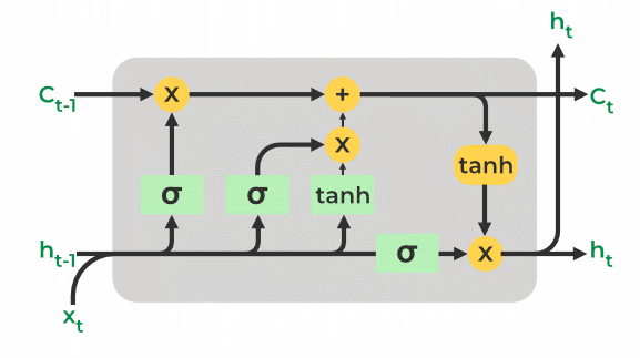
LSTM Model architecture

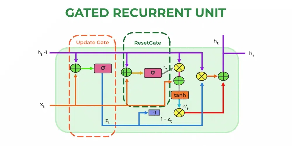
49. What is GRU? and How it works?

Ans: GRU stands for Gated Recurrent Unit. GRUs are recurrent neural networks (RNNs) that can process sequential data such as text, audio, or time series.GRU uses gating mechanisms to control the flow of information in and out of the network, allowing it to learn from the temporal dependencies in the data and adjust its behaviour accordingly.

GRU is similar to LSTM in that it uses gating mechanisms, but it has a simpler architecture with fewer gates, making it computationally more efficient and easier to train. It uses two types of Gates: the reset gate (r) and the update gate (z)

1. Rest Gate (r): It determines which parts of the previous hidden state should be forgotten or reset. It takes The update gate decides which parts of the current hidden state should be updated with new information from the current input. Similar to the reset gate, it takes the previous hidden state and the current input as inputs and outputs a value between 0 and 1 for each element of the hidden state.
   
2. Update Gate (z): It decides which part of the current hidden state should be updated with the new information from the current input. It takes the previous hidden state and the current input as inputs and the outputs value between 0 and 1 for each element of the hidden state.
   

GRU models have been demonstrated to be useful in NLP applications such as language modelling, sentiment analysis, machine translation, and text generation. They are especially beneficial when it is critical to record long-term dependencies and grasp the context. GRU is a popular choice in NLP research and applications due to its simplicity and computational efficiency.

50. What is an Encoder-Decoder network in Deep Learning?

An encoder-decoder network is a kind of neural network that can learn to map an input sequence to a different length and structure output sequence. It is made up of two primary parts: an encoder and a decoder.

• Encoder: The encoder takes a variable-length input sequence (such as a sentence, an image, or a video) and processes it step by step steps to build a fixed-length context or encoded vector or representation that captures the important information from the input sequence. The encoded vector condenses the information from the entire input sequence.
• Decoder: Decoder is another neural network that takes the encoded vector as input and generates an output sequence (such as another sentence, an image, or a video) that is related to the input sequence. The decoder generates an output and modifies its internal hidden state based on the encoded vector and previously generated outputs at each step.

The training process of an Encoder-Decoder network involves feeding pairs of input and target sequences to the model and minimizing the difference between the predicted output sequence and the true target sequence using a suitable loss function. Encoder-Decoder networks are used for a variety of tasks, such as machine translation (translating text from one language to another), text summarization, chatbots, and image captioning (turning pictures into meaningful phrases).

51. What is an autoencoder?

Autoencoders are a type of neural network architecture used for unsupervised learning tasks like dimensionality reduction, feature learning, etc. Autoencoders work on the principle of learning a low-dimensional representation of high-dimensional input data by compressing it into a latent representation and then reconstructing the input data from the compressed representation. It consists of two main parts an encoder and a decoder.  The encoder maps an input to a lower-dimensional latent representation, while the decoder maps the latent representation back to the original input space. In most cases, neural networks are used to create the encoder and decoder, and they are trained in parallel to reduce the difference between the original input data and the reconstructed data.

52. What is a Generative Adversarial Network (GAN)?

Generative Adversarial Networks (GANs) are a type of neural network architecture used for unsupervised learning tasks like image synthesis and generative modeling. It is composed of two neural networks: Generator and Discriminator. The generator takes the random distributions mainly the Gaussian distribution as inputs and generates the synthetic data, while the discriminator takes both real and synthetic data as input and predicts whether the input is real or synthetic. The goal of the generator is to generate synthetic data that is identical to the input data. and the discriminator guesses whether the input data is real or synthetic.

53. What is the attention mechanism?

An attention mechanism is a type of neural network that employs a separate attention layer within an Encoder-Decoder neural network to allow the model to focus on certain areas of the input while executing a task. It accomplishes this by dynamically assigning weights to various input components, reflecting their relative value or relevance. This selective attention enables the model to concentrate on key information, capture dependencies, and understand data linkages.

The attention mechanism is especially useful for tasks that need sequential or structured data, such as natural language processing, where long-term dependencies and contextual information are critical for optimal performance. It allows the model to selectively attend the important features or contexts, which increases the model’s capacity to manage complicated linkages and dependencies in the data, resulting in greater overall performance in various tasks.

54. What is the Transformer model?

Transformer is an important model in neural networks that relies on the attention mechanism, allowing it to capture long-range dependencies in sequences more efficiently than typical RNNs. It has given state-of-the-art results in various NLP tasks like word embedding, machine translation, text summarization, question answering etc.

The key components of the Transformer model are as follows:

• Self-Attention Mechanism: A self-attention mechanism is a powerful tool that allows the Transformer model to capture long-range dependencies in sequences. It allows each word in the input sequence to attend to all other words in the same sequence, and the model learns to assign weights to each word based on its relevance to the others. This enables the model to capture both short-term and long-term dependencies, which is critical for many NLP applications.
• Encoder-Decoder Network: An encoder-decoder architecture is used in the Transformer model. The encoder analyzes the input sequence and creates a context vector that contains information from the entire sequence. The context vector is then used by the decoder to construct the output sequence step by step.
• Multi-head Attention: The purpose of the multi-head attention mechanism in Transformers is to allow the model to recognize different types of correlations and patterns in the input sequence. In both the encoder and decoder, the Transformer model uses multiple attention heads. This enables the model to recognise different types of correlations and patterns in the input sequence. Each attention head learns to pay attention to different parts of the input, allowing the model to capture a wide range of characteristics and dependencies.
• Positional Encoding: Positional encoding is applied to the input embeddings to offer this positional information like the relative or absolute position of each word in the sequence to the model. These encodings are typically learnt and can take several forms, including sine and cosine functions or learned embeddings. This enables the model to learn the order of the words in the sequence, which is critical for many NLP tasks.
• Feed-Forward Neural Networks: Following the attention layers, the model applies a point-wise feed-forward neural network to each position separately. This enables the model to learn complex non-linear correlations in the data.
• Layer Normalization and Residual Connections: Layer normalization is used to normalize the activations at each layer of the Transformer, promoting faster convergence during training. Furthermore, residual connections are used to carry the original input directly to successive layers, assisting in mitigating the vanishing gradient problem and facilitating gradient flow during training.

55. What is Transfer Learning?

Transfer learning is a machine learning approach that involves implementing the knowledge and understanding gained by training a model on one task and applying that knowledge to another related task. The basic idea behind transfer learning is that a model that has been trained on a big, diverse dataset may learn broad characteristics that are helpful for many different tasks and can then be modified or fine-tuned to perform a specific task with a smaller, more specific dataset.

Transfer learning can be applied in the following ways:

1. Fine-tuning: Fine-tuning is used to adapt a pre-trained model that has already been trained on a big dataset and refine it with further training on a new smaller dataset that is specific to the present task. With fine-tuning, weights of the pre-trained model can be adjusted according to the new present task while training on the new dataset. This can improve the performance of the model on the new task.
2. Feature extraction: In this case, the features of the pre-trained model are extracted, and these extracted features can be used as the input for the new model. This can be useful when the new task involves a different input format than the original task.
3. Domain adaptation:  In this case, A pre-trained model is adapted from a source domain to a target domain by modifying its architecture or training process to better fit the target domain.
4. Multi-task learning: By simultaneously training a single network on several tasks, this method enables the network to pick up common representations that are applicable to all tasks.
5. One-shot learning: This involves applying information gained from previous tasks to train a model on just one or a small number of samples of a new problem.

56. What are distributed and parallel training in deep learning?

Deep learning techniques like distributed and parallel training are used to accelerate the training process of bigger models. Through the use of multiple computing resources, including CPUs, GPUs, or even multiple machines, these techniques distribute the training process in order to speed up training and improve scalability.

When storing a complete dataset or model on a single machine is not feasible, multiple machines must be used to store the data or model. When the model is split across multiple machines, then it is known as model parallelism. In model parallelism, different parts of the model are assigned to different devices or machines. Each device or machine is responsible for computing the forward and backward passes for the part of the model assigned to it.

When the data is too big that it is distributed across multiple machines, it is known as data parallelism. Distributed training is used to simultaneously train the model on multiple devices, each of which processes a separate portion of the data. In order to update the model parameters, the results are combined, which speed-up convergence and improve the performance of the model.

Parallel training, involves training multiple instances of the same model on different devices or machines. Each instance trains on a different subset of the data and the results are combined periodically to update the model parameters. This technique can be particularly useful for training very large models or dealing with very large datasets.

Both parallel and distributed training need specialized hardware and software configurations, and performance may benefit from careful optimization. However, they may significantly cut down on the amount of time needed to train deep neural networks.

Conclusion

At the end, in order to prepare deep learning interview questions, one must first review its fundamental concepts and get a thorough basic understanding of the patterns of frequently asked questions. One needs to practice well to feel confident in answering the interview questions. Overall, everything that is frequently asked was addressed in this article, but for a better understanding, prepare well in advance through projects and practising problems.