Decision Tree for Regression in R Programming
Last Updated :
28 Jul, 2020
Decision tree is a type of algorithm in machine learning that uses decisions as the features to represent the result in the form of a tree-like structure. It is a common tool used to visually represent the decisions made by the algorithm. Decision trees use both classification and regression. Regression trees are used when the dependent variable is continuous whereas the classification tree is used when the dependent variable is categorical. For example, determining/predicting gender is an example of classification, and predicting the mileage of a car based on engine power is an example of regression. In this article, let us discuss the decision tree using regression in R programming with syntax and implementation in R programming.
Implementation in R
In R programming, rpart() function is present in rpart package. Using the rpart() function, decision trees can be built in R.
Syntax:
rpart(formula, data, method)
Parameters:
formula: indicates the formula based on which model has to be fitted
data: indicates the dataframe
method: indicates the method to create decision tree. “anova” is used for regression and “class” is used as method for classification.
Example 1:
In this example, let us predict the sepal width using the regression decision tree.
Step 1: Install the required package
install.packages("rpart")
|
Step 2: Load the package
Step 3: Fit the model for decision tree for regression
fit <- rpart(Sepal.Width ~ Sepal.Length +
Petal.Length + Petal.Width + Species,
method = "anova", data = iris)
|
Step 4: Plot the tree
png(file = "decTreeGFG.png", width = 600,
height = 600)
plot(fit, uniform = TRUE,
main = "Sepal Width Decision
Tree using Regression")
text(fit, use.n = TRUE, cex = .7)
dev.off()
|
Step 5: Print the decision tree model
Step 6: Predicting the sepal width
df <- data.frame (Species = 'versicolor',
Sepal.Length = 5.1,
Petal.Length = 4.5,
Petal.Width = 1.4)
cat("Predicted value:\n")
predict(fit, df, method = "anova")
|
Output:
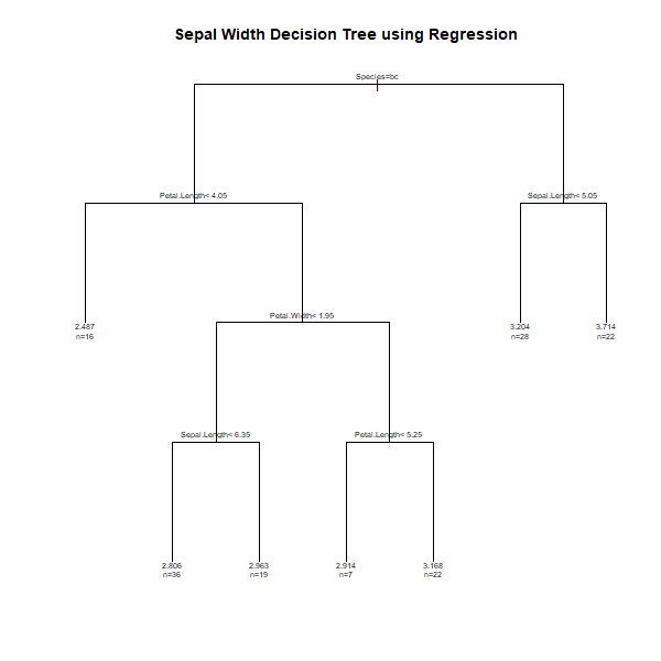
n= 150

node), split, n, deviance, yval
      * denotes terminal node

 1) root 150 28.3069300 3.057333
   2) Species=versicolor, virginica 100 10.9616000 2.872000
     4) Petal.Length=4.05 84  7.3480950 2.945238
      10) Petal.Width< 1.95 55  3.4920000 2.860000
        20) Sepal.Length=6.35 19  0.6242105 2.963158 *
      11) Petal.Width>=1.95 29  2.6986210 3.106897
        22) Petal.Length=5.25 22  2.0277270 3.168182 *
   3) Species=setosa 50  7.0408000 3.428000
     6) Sepal.Length=5.05 22  1.7859090 3.713636 *

Predicted value:
       1
2.805556
Example 2:
In this example, let us predict the mpg value using a decision tree for regression.
Step 1: Install the required package
install.packages("rpart")
|
Step 2: Load the package
Step 3: Fit the model for decision tree for regression
fit <- rpart(mpg ~ disp + hp + cyl,
method = "anova", data = mtcars )
|
Step 4: Plot the tree
png(file = "decTree2GFG.png", width = 600,
height = 600)
plot(fit, uniform = TRUE,
main = "MPG Decision Tree using Regression")
text(fit, use.n = TRUE, cex = .6)
dev.off()
|
Step 5: Print the decision tree model
Step 6: Predicting the mpg value using test dataset
df <- data.frame (disp = 351, hp = 250,
cyl = 8)
cat("Predicted value:\n")
predict(fit, df, method = "anova")
|
Output:
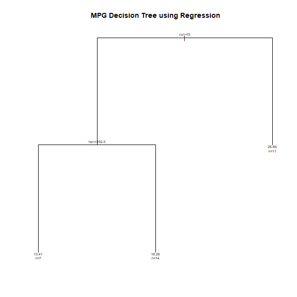
n= 32

node), split, n, deviance, yval
      * denotes terminal node

1) root 32 1126.04700 20.09062
  2) cyl>=5 21  198.47240 16.64762
    4) hp>=192.5 7   28.82857 13.41429 *
    5) hp< 192.5 14   59.87214 18.26429 *
  3) cyl< 5 11  203.38550 26.66364 *

Predicted value:
       1
13.41429
Advantages of Decision Trees
- Considers all the possible decisions: Decision trees considers all the possible decisions to create a result of the problem.
- Easy to use: With classification and regression techniques, it is easy to use for any type of problem and further creating predictions and solving the problem.
- No problem with missing values: There is no problem with the datasets having missing values and do not affect the decision tree building.
Disadvantages of Decision Trees
- Requires higher time: Decision trees requires higher time for the calculation for large datasets.
- Less learning: Decision trees are not good learners. Random forest approach is used for better learning.
Like Article
Suggest improvement
Share your thoughts in the comments
Please Login to comment...