Data Science | Solving Linear Equations

Linear Algebra is a very fundamental part of Data Science. When one talks about Data Science, data representation becomes an important aspect of Data Science. Data is represented usually in a matrix form. The second important thing in the perspective of Data Science is if this data contains several variables of interest, then one is interested to know how many of these are very important. And if there are relationships between these variables, then how can one uncover these relationships? 

You can go through the Introduction to Data Science: Skills Required article to have a basic understanding of what Data Science is?

Linear algebraic tools allow us to understand these data. So, a Data Science enthusiast needs to have a good understanding of this concept before going to understand complex machine learning algorithms.

Matrices and Linear Algebra

There are many ways to represent the data, matrices provide you with a convenient way to organize these data. 

• Matrices can be used to represent samples with multiple attributes in a compact form
• Matrices can also be used to represent linear equations in a compact and simple fashion
• Linear algebra provides tools to understand and manipulate matrices to derive useful knowledge from data

Identification of Linear Relationships Among Attributes
We identify the linear relationship between attributes using the concept of null space and nullity. Before proceeding further, go through Null Space and Nullity of a Matrix.
Preliminaries

Generalized linear equations are represented as below: Ax=b

Where,

• A is an mXn matrix
• x is nX1 variables or unknown terms
• b is the dependent variable mX1
• m & n are the numbers of equations and variables

In general, there are three cases one needs to understand: 

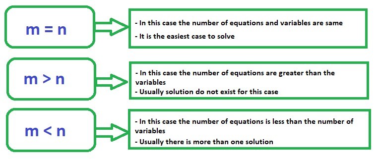
We will consider these three cases independently.
Full row rank and full column rank
For a matrix A (m x n)

Full Row Rank	Full Column Rank
When all the rows of the matrix are linearly independent,	When all the columns of the matrix are linearly independent,
Linearly independent rows mean no row can be expressed as a linear combination of the other rows. In other words, every row contributes uniquely to the overall information in the matrix. If a matrix has full row rank, the number of linearly independent rows is equal to the number of columns in the matrix.	Linearly independent columns mean no column can be expressed as a linear combination of the other columns. In this case, each column carries unique information in the matrix. If a matrix has full column rank, the number of linearly independent columns is equal to the number of rows in the matrix.
Data sampling does not present a linear relationship – samples are independent	Attributes are linearly independent

Note: In general whatever the size of the matrix it is established that the row rank is always equal to the column rank. It means for any size of the matrix if we have a certain number of independent rows, we will have those many numbers of independent columns. 
In general case, if we have a matrix m x n and m is smaller than n then the maximum rank of the matrix can only be m. So, the maximum rank is always the less of the two numbers m and n. 

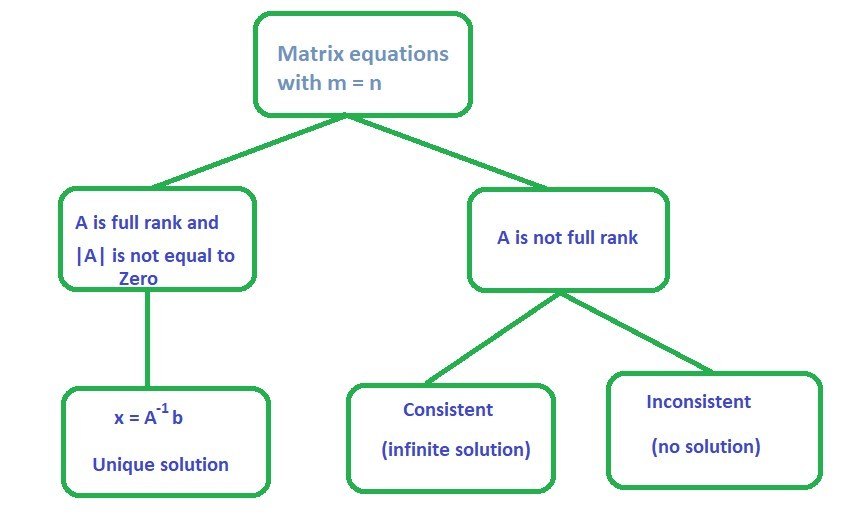
Case 1: m = n

The solution for this type of linear equation if A is a full rank matrix having determinant of A is equal to 0 will be:

[Tex]\begin{aligned} Ax&=b \\ x &= A^{-1}b \end{aligned}[/Tex]

Example 1.1:

Consider the given matrix equation:

[Tex]\begin{bmatrix} 1&3\\ 2&4\\ \end{bmatrix} % \begin{bmatrix} x_1\\ x_2\\ \end{bmatrix} = \begin{bmatrix} 7\\ 10\\ \end{bmatrix}[/Tex]

• |A| is not equal to zero
• rank(A) = 2 = no. of columns this implies that A is full rank

[Tex]\begin{aligned} \begin{bmatrix} x_1\\ x_2\\ \end{bmatrix} &= \begin{bmatrix} 1&3\\ 2&4\\ \end{bmatrix}^{-1} \begin{bmatrix} 7\\ 10\\ \end{bmatrix} \\&= \begin{bmatrix} -2&1.5\\ 1&-0.5\\ \end{bmatrix} \begin{bmatrix} 7\\ 10\\ \end{bmatrix} \\&= \begin{bmatrix} 1\\ 2\\ \end{bmatrix} \end{aligned}[/Tex]

Therefore, the solution for the given example is [Tex](x_1, x_2) = (1, 2)    [/Tex]    

Example 1.2:

Consider the given matrix equation:

[Tex]\begin{bmatrix} 1&2\\ 2&4\\ \end{bmatrix} % \begin{bmatrix} x_1\\ x_2\\ \end{bmatrix} = \begin{bmatrix} 5\\ 10\\ \end{bmatrix}[/Tex]

• |A| is not equal to zero 
• rank(A) = 1nullity = 1

Checking consistency

[Tex]\begin{bmatrix} x_1 + 2x_2\\ 2x_1 + 4x_2\\ \end{bmatrix} = \begin{bmatrix} 5\\ 10\\ \end{bmatrix}[/Tex]

• Row (2) = 2 
• Row (1)
• The equations are consistent with only one linearly independent equation
• The solution set for (x_1, x_2) is infinite because we have only one linearly independent equation and two variables    

Explanation: In the above example we have only one linearly independent equation i.e. [Tex]x_1+2x_2 = 5    [/Tex]. So, if we take [Tex]x_2 = 0    [/Tex], then we have [Tex]x_1 = 5    [/Tex]; if we take [Tex]x_2 = 1    [/Tex], then we have [Tex]x_1 = 3    [/Tex]. In a similar fashion, we can have many solutions to this equation. We can take any value of [Tex]x_2        [/Tex]( we have infinite choices for [Tex]x_2        [/Tex]) and correspondingly for each value of [Tex]x_2        [/Tex]we will get one [Tex]x_1        [/Tex]. Hence, we can say that this equation has infinite solutions.

Example 1.3:

Consider the given matrix equation:

[Tex]\begin{bmatrix} 1&2\\ 2&4\\ \end{bmatrix} \begin{bmatrix} x_1\\ x_2\\ \end{bmatrix} = \begin{bmatrix} 5\\ 9\\ \end{bmatrix} [/Tex]

• |A| is not equal to zero
• rank(A) = 1
• nullity = 1

Checking consistency

[Tex]\begin{bmatrix} x_1 + 2x_2\\ 2x_1 + 4x_2\\ \end{bmatrix} = \begin{bmatrix} 5\\ 9\\ \end{bmatrix} [/Tex]

2 Row (1) = [Tex]2x_1 + 4x_2 = 10 \neq 9 [/Tex]

Therefore, the equations are inconsistent

We cannot find the solution to ([Tex]x_1, x_2    [/Tex])

Case 2: m > n

• In this case, the number of variables or attributes is less than the number of equations.
• Here, not all the equations can be satisfied.
• So, it is sometimes termed as a case of no solution.
• But, we can try to identify an appropriate solution by viewing this case from an optimization perspective.

An optimization perspective

-Rather than finding an exact solution of a system of linear equations Ax = b, we can find an [Tex]x   [/Tex] such that (Ax-b) can be minimized.

Here, Ax-b is a vector. 

There will be as many error terms as the number of equations- Denote Ax-b = e (m x 1); there are m errors e_i, i = 1:m- We can minimize all the errors collectively by minimizing [Tex]\sum_{i=1}^{m} e_i^{2}-   [/Tex] This is the same as minimizing (Ax-b)^{T}(Ax-b)

So, the optimization problem becomes 

[Tex]\begin{aligned} \sum_{i=1}^{m} e_i^{2}&=min[(Ax-b)^{T}(Ax-b)] \\&=min[(x^{T}A^{T}-b^{T})(Ax-b)] \\&=min[x^{T}A^{T}Ax-b^{T}Ax-x^{T}A^{T}b+b^{T}b] &\\&=f(x) \end{aligned}[/Tex]

Here, we can notice that the optimization problem is a function of x. When we solve this optimization problem, it will give us the solution for x. We can obtain the solution to this optimization problem by differentiating [Tex]f(x)   [/Tex]with respect to x and setting the differential to zero.

[Tex] \nabla f(x) = 0 [/Tex]

– Now, differentiating f(x) and setting the differential to zero results in 

[Tex]\begin{aligned} \nabla f(x) &= 0 \\ 2(A^{T}A)x – 2A^{T}b &= 0 \\A^{T}Ax &= A^{T}b   \end{aligned}[/Tex]

– Assuming that all the columns are linearly independent 

[Tex]x = (A^{T}A)^{-1}A^{T}b     [/Tex]

Note: While this solution x might not satisfy all the equations but it will ensure that the errors in the equations are collectively minimized.

Example 2.1:

Consider the given matrix equation:

[Tex]\begin{bmatrix} 1&0\\ 2&0\\ 3&1\\ \end{bmatrix} % \begin{bmatrix} x_1\\ x_2\\ \end{bmatrix} = \begin{bmatrix} 1\\ -0.5\\ 5\\ \end{bmatrix}[/Tex]

• m = 3, 
• n = 2

Using the optimization concept

[Tex]\begin{aligned} x &= (A^{T}A)^{-1}A^{T}b \\\begin{bmatrix} x_1\\ x_2\\ \end{bmatrix} &= \begin{bmatrix} 0.2&-0.6\\ -0.6&2.8 \\ \end{bmatrix} \begin{bmatrix} 15\\ 5\\ \end{bmatrix} \\ &= \begin{bmatrix} 0\\ 5\\ \end{bmatrix} \end{aligned}[/Tex]

Therefore, the solution for the given linear equation is [Tex](x_1, x_2) = (0, 5)[/Tex]

Substituting in the equation shows

[Tex]\begin{bmatrix} 1&0\\ 2&0\\ 3&1\\ \end{bmatrix} % \begin{bmatrix} 0\\ 5\\ \end{bmatrix} = \begin{bmatrix} 0\\ 0\\ 5\\ \end{bmatrix} \neq \begin{bmatrix} 1\\ -0.5\\ 5\\ \end{bmatrix}[/Tex]

Example 2.2:

Consider the given matrix equation:

[Tex]\begin{bmatrix} 1&0\\ 2&0\\ 3&1\\ \end{bmatrix} % \begin{bmatrix} x_1\\ x_2\\ \end{bmatrix} = \begin{bmatrix} 1\\ 2\\ 5\\ \end{bmatrix}[/Tex]

• m = 3, 
• n = 2

Using the optimization concept

[Tex]\begin{aligned} x &= (A^{T}A)^{-1}A^{T}b \\ \begin{bmatrix} x_1\\ x_2\\ \end{bmatrix} &= \begin{bmatrix} 0.2&-0.6\\ -0.6&2.8\\ \end{bmatrix} \begin{bmatrix} 20\\ 5\\ \end{bmatrix} \\ &= \begin{bmatrix} 1\\ 2\\ \end{bmatrix} \end{aligned}[/Tex]

Therefore, the solution for the given linear equation is [Tex](x_1, x_2) = (1, 2)[/Tex]

Substituting in the equation shows:

[Tex]\begin{bmatrix} 1&0\\ 2&0\\ 3&1\\ \end{bmatrix} % \begin{bmatrix} 1\\ 2\\ \end{bmatrix} = \begin{bmatrix} 1\\ 2\\ 5\\ \end{bmatrix} = \begin{bmatrix} 1\\ 2\\ 5\\ \end{bmatrix}[/Tex]

So, the important point to notice in case 2 is that if we have more equations than variables then we can always use the least square solution which is [Tex]x = (A^{T}A)^{-1}A^{T}b   [/Tex]. 

There is one thing to keep in mind is that [Tex](A^{T}A)^{-1}   [/Tex] exists if the columns of A are linearly independent.

Case 3: m < n

• This case deals with more number of attributes or variables than equations
• Here, we can obtain multiple solutions for the attributes
• This is an infinite solution case.
• We will see how we can choose one solution from the set of infinite possible solution

In this case, also we have an optimization perspective. Know what is Lagrange function here. 

– Given below is the optimization problem  [Tex]min\left[ \frac{1}{2}x^{T}x \right]   [/Tex] 

such that, Ax=b

– We can define a Lagrangian function 

[Tex]min[ f(x, \lambda)] =min\left[ \frac{1}{2}x^{T}x + \lambda^{T}(Ax-b) \right]     [/Tex]

– Differentiate the Lagrangian with respect to x, and set it to zero, then we will get, 

[Tex]\begin{aligned} x + A^{T}\lambda &= 0  \\ x &= -A^{T}\lambda  \end{aligned}[/Tex]

Pre – multiplying by A 

[Tex]\begin{aligned} Ax&=b \\A(-A^{T}\lambda) &= b \\ -AA^{T}\lambda&=b \\ \lambda &= -(AA^{T})^{-1}b \end{aligned}[/Tex]

assuming that all the rows are linearly independent 

[Tex]\begin{aligned} x &= -A^{T}\lambda \\ &= A^{T}(AA^{T})^{-1}b \end{aligned}[/Tex]

Example 3.1:

Consider the given matrix equation:

[Tex]\begin{bmatrix} 1&2&3\\ 0&0&1\\ \end{bmatrix} % \begin{bmatrix} x_1\\ x_2\\ x_3\\ \end{bmatrix} = \begin{bmatrix} 2\\ 1\\ \end{bmatrix}[/Tex]

• m = 2, 
• n = 3

Using the optimization concept

[Tex]\begin{aligned} x &= A^{T}(AA^{T})^{-1}b \\ &= \begin{bmatrix} 1&0\\ 2&0\\ 3&1\\ \end{bmatrix} \left( \begin{bmatrix} 1&2&3\\ 0&0&1\\ \end{bmatrix} \begin{bmatrix} 1&0\\ 2&0\\ 3&1\\ \end{bmatrix} \right )^{-1} \begin{bmatrix} 2\\ 1\\ \end{bmatrix} \\ &= \begin{bmatrix} 1&0\\ 2&0\\ 3&1\\ \end{bmatrix} \begin{bmatrix} -0.2\\ 1.6\\ \end{bmatrix} \\ \begin{bmatrix} x_1\\ x_2\\ x_3\\ \end{bmatrix} &= \begin{bmatrix} -0.2\\ -0.4\\ 1\\ \end{bmatrix} \end{aligned}[/Tex]

The solution for the given sample is ([Tex]x_1, x_2, x_3   [/Tex]) = (-0.2, -0.4, 1)

You can easily verify that

 [Tex]\begin{bmatrix} 1&0\\ 2&0\\ 3&1\\ \end{bmatrix} % \begin{bmatrix} x_1\\ x_2\\ x_3\\ \end{bmatrix} = \begin{bmatrix} 2\\ 1\\ \end{bmatrix}[/Tex]

Generalization

• The above-described cases cover all the possible scenarios that one may encounter while solving linear equations.
• The concept we use to generalize the solutions for all the above cases is called Moore – Penrose Pseudoinverse of a matrix.
• Singular Value Decomposition can be used to calculate the psuedoinverse or the generalized inverse ([Tex]A^+        [/Tex]).