Data Mining in R

Data mining is the process of discovering patterns and relationships in large datasets. It involves using techniques from a range of fields, including machine learning, statistics, and database systems, to extract valuable insights and information from data.

R is a popular programming language for data analysis and statistical computing and is well-suited for data mining tasks. It has a large and active community of users and developers, which has resulted in a rich ecosystem of packages and tools for data mining.

In this article, we will provide an overview of data mining in the R Programming Language, including some of the most commonly used techniques and tools. We will begin by introducing the basics of data mining and R and then delve into more advanced topics such as machine learning, text mining, and social network analysis.

Getting started with data mining in R

To begin data mining in R, you will need to install the language and a development environment. There are several options available, including the RStudio IDE, which is widely used by R users and offers a range of features for data mining and other tasks.

Once you have installed R and a development environment, you can start exploring the vast array of packages and tools available for data mining. Some of the most popular packages for data mining in R include:

• caret: This package provides a range of functions for training and evaluating machine learning models in R.
• dplyr: This package provides a set of functions for data manipulation, including filtering, grouping, and summarizing data.
• ggplot2: This package is a popular tool for data visualization in R, and can be used to create a wide range of plots and charts.
• tm: This package provides tools for text mining, including functions for preprocessing and analyzing text data.
• igraph: This package is a powerful tool for analyzing and visualizing network data, including social networks.

These are just a few examples of the many packages available for data mining in R. To get started with any of these packages, you can install them using the install.packages() function and then load them into your R session using the library() function.

Data preparation

Before you can begin data mining, you will need to obtain and prepare your data. This process, known as data preprocessing, involves a range of tasks including cleaning, transforming and integrating data from various sources.

In R, there are a number of packages and functions available for data preprocessing. Some examples include:

• read.csv(): This function reads a CSV (comma-separated values) file into R as a data frame.
• tidyr: This package provides functions for reshaping and restructuring data, such as gather() and spread() for converting between wide and long data formats.
• dplyr: As mentioned previously, this package provides a range of functions for data manipulation, including filter() for selecting rows based on specific criteria, group_by() for grouping data by certain variables, and summarize() for computing summary statistics.

It is important to carefully consider the quality and relevance of your data before beginning any data mining tasks. Poor quality data can lead to incorrect or misleading results, so it is worth investing time and effort in cleaning and preparing your data.

Exploratory data analysis

Once your data is prepared, you can begin exploring and visualizing it to gain insights and understand the underlying patterns and relationships. This process, known as exploratory data analysis (EDA), is an important step in the

Feature selection: This involves selecting a subset of the available variables or features in your data to use in your analysis. There are various techniques for feature selection, including filtering, wrapper methods, and embedded methods.

Dimensionality Reduction

This involves reducing the number of dimensions or variables in your data, either by projecting the data onto a lower-dimensional space or by combining variables in some way. Techniques for dimensionality reduction include principal component analysis (PCA) and multidimensional scaling (MDS).

R

# Loading the package
install.packages("dplyr")
library(dplyr)

# Loading Data
data(mtcars)

# Apply PCA using prcomp function
# Need to scale / Normalize as
# PCA depends on distance measure
my_pca <- prcomp(mtcars, scale = TRUE,
                center = TRUE, retx = T)
names(my_pca)

# Summary
summary(my_pca)

Output:

'sdev''rotation''center''scale''x'

Importance of components:
                          PC1    PC2     PC3     PC4     PC5     PC6    PC7
Standard deviation     2.5707 1.6280 0.79196 0.51923 0.47271 0.46000 0.3678
Proportion of Variance 0.6008 0.2409 0.05702 0.02451 0.02031 0.01924 0.0123
Cumulative Proportion  0.6008 0.8417 0.89873 0.92324 0.94356 0.96279 0.9751
                           PC8    PC9    PC10   PC11
Standard deviation     0.35057 0.2776 0.22811 0.1485
Proportion of Variance 0.01117 0.0070 0.00473 0.0020
Cumulative Proportion  0.98626 0.9933 0.99800 1.0000

Clustering

This involves partitioning a dataset into groups (called clusters) such that the observations within each cluster are more similar to each other than they are to observations in other clusters. Clustering can be used for a variety of purposes, including discovering hidden patterns in the data, summarizing data, and generating new features.

R

# Library required for fviz_cluster function
install.packages("factoextra")
library(factoextra)

# Loading dataset
df <- mtcars

# Omitting any NA values
df <- na.omit(df)

# Scaling dataset
df <- scale(df)

# output to be present as PNG file
png(file = "KMeansExample.png")

km <- kmeans(df, centers = 4, nstart = 25)

# Visualize the clusters
fviz_cluster(km, data = df)

# saving the file
dev.off()

# output to be present as PNG file
png(file = "KMeansExample2.png")

km <- kmeans(df, centers = 5, nstart = 25)

# Visualize the clusters
fviz_cluster(km, data = df)

# saving the file
dev.off()

Output:

Clusters formed using 4 cluster centers

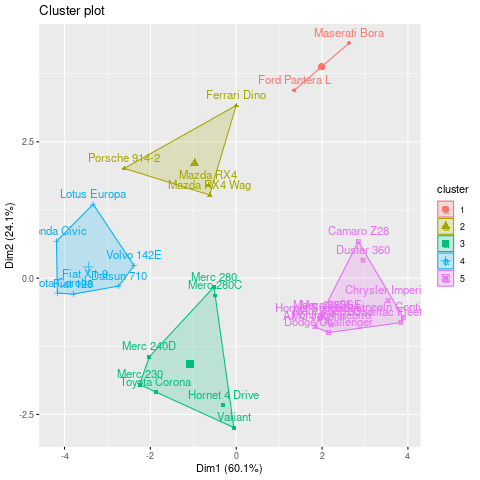
Clusters formed using 5 cluster centers

Association Rule Mining

This involves discovering frequent patterns or associations in the data, such as items that are frequently purchased together in a retail setting. Association rule mining is often used in market basket analysis and recommendation systems.

Outlier Detection

This involves identifying observations in the data that are significantly different from the majority of the data and may indicate errors or anomalies. Outlier detection can be useful for identifying problems with the data or identifying unusual observations that warrant further investigation.

R

data <- rnorm(500)

data[1:10] <- c(-4, 2, 5, 6, 4,
                1, -5, 8, 9, -6)

boxplot(data)

Output:

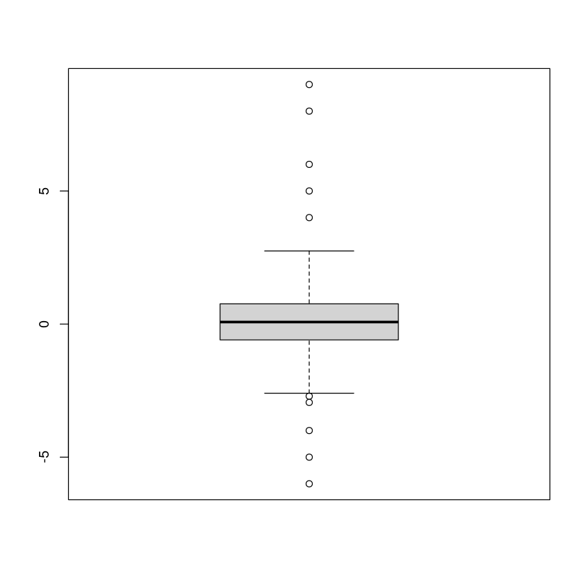
Points that are outside the whiskers of the boxplot are considered as outliers

Data Mining and Text Mining Process

The data mining process typically involves several steps, including data preparation, exploratory data analysis, model building, evaluation, and deployment. Text mining involves extracting and analyzing text data, often with the goal of uncovering patterns and relationships within the text. Text mining can be used to analyze social media data, customer reviews, and other types of unstructured text data.

Machine Learning

Machine learning is a subset of artificial intelligence that involves building models that can learn from data and make predictions or decisions. There are many different types of machine learning algorithms, including decision trees, neural networks, and support vector machines.

Data Visualization

Data visualization is the process of creating charts, plots, and other visual representations of data in order to understand and communicate the underlying patterns and relationships. There are many packages and tools available for data visualization in R, including ggplot2, lattice, and Plotly.

Regression

Linear Regression is one of the most widely used regression techniques to model the relationship between two variables. It uses a linear relationship to model the regression line. There are 2 variables used in the linear relationship equation i.e., the predictor variable and the response variable.

Linear Regression Equation:

y = a x + b

where,

• x indicates predictor or independent variable
• y indicates response or dependent variable
• a and b are coefficients

R

# R program to illustrate
# Linear Regression

# Height vector
x <- c(153, 169, 140, 186, 128,
    136, 178, 163, 152, 133)

# Weight vector
y <- c(64, 81, 58, 91, 47, 57,
    75, 72, 62, 49)

# Create a linear regression model
model <- lm(y~x)

# Print regression model
print(model)

# Find the weight of a person
# With height 182
df <- data.frame(x = 182)
res <- predict(model, df)
cat("\nPredicted value of a person
            with height = 182")
print(res)

# Output to be present as PNG file
png(file = "linearRegGFG.png")

# Plot
plot(x, y, main = "Height vs Weight
                Regression model")
abline(lm(y~x))

# Save the file.
dev.off()

Output:

Coefficients:
(Intercept)            x  
   -39.7137       0.6847

Predicted value of a person with height = 182
      1 
84.9098

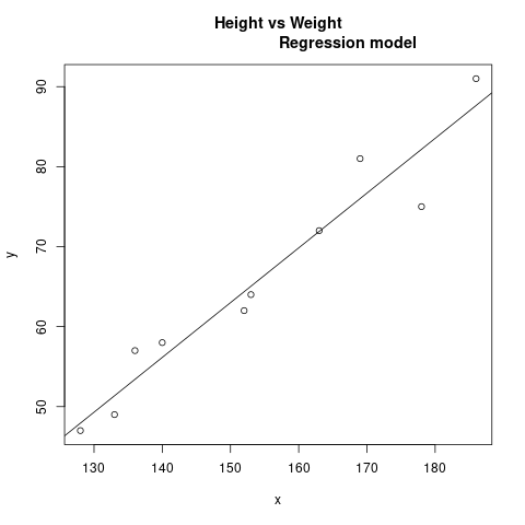
Regression line with the points on a 2D plot

Classification

Classification is a supervised learning approach in which data is classified on the basis of the features provided. As in the above example, data is being classified in different parameters using random forest. It helps in creating more meaningful observations or classifications. In simple words, classification is a way of categorizing structured or unstructured data into some categories or classes. Now let’s try to build a random forest classification model using the iris dataset.

R

# Load the library
library(randomForest)

# Create random forest for classification
iris.rf <- randomForest(Species ~ .,
                        data = iris,
                        importance = TRUE,
                        proximity = TRUE)

# Print classification model
print(iris.rf)

Output:

               Type of random forest: classification
                     Number of trees: 500
No. of variables tried at each split: 2

        OOB estimate of  error rate: 5.33%
Confusion matrix:
           setosa versicolor virginica class.error
setosa         50          0         0        0.00
versicolor      0         47         3        0.06
virginica       0          5        45        0.10

Data Preprocessing

Data preprocessing involves a range of tasks that are performed on raw data in order to prepare it for analysis. This can include cleaning, filtering, transforming, and integrating data from multiple sources.

Data Mining Necessary Steps

Here are the general steps involved in the data mining process:

1. Define the problem and objectives: Before beginning the data mining process, it is important to clearly define the problem you are trying to solve and the specific objectives you are trying to achieve.
2. Collect and prepare the data: This step involves acquiring and preparing the data for analysis. This can include cleaning and preprocessing the data, as well as selecting a subset of the data to focus on.
3. Explore and visualize the data: In this step, you will explore and visualize the data in order to gain a better understanding of the patterns and relationships present in the data. This can involve creating charts, plots, and other visualizations to help you identify trends and outliers.
4. Build and evaluate models: In this step, you will use machine learning algorithms and other techniques to build models that can analyze the data and make predictions or decisions. You will also need to evaluate the performance of the models and fine-tune them as needed.
5. Deploy and maintain the models: Once you have built and evaluated your models, you will need to deploy them in a production environment and ensure that they are functioning correctly. You may also need to periodically update and maintain the models as the data or business requirements change.