Custom Format to Show Units Without Changing Number to Text in Excel

Microsoft Excel is a great software that is used by individuals to store data in the form of spreadsheets in a formatted manner. Microsoft Excel allows us to store a variety of data such as characters, text, numbers, decimals, date, time, etc. Since Excel is a smart tool, it automatically identifies the data type of the records and places them accordingly inside the cell based on its default convention. But, there can be scenarios in which we want to store data which is actually of kind number but along with some unit which is generally text. Let’s say we want to store unit values like 10 Litres (10 L), 20 Litres (20 L) or we want to store distance traveled like 2 km, 5 km. In such cases, when we input let’s say 2 km or 20 L inside a cell then it will be treated as a text by Excel automatically. But, what if we want these records to be actually stored as numbers inside the cell, so that we can perform some functional operations on these numbers such as calculating the total amount of currency or calculating the total distance traveled. In such cases, mathematical formulas cannot be performed on text values. Hence, we are required to change those texts back to numbers. In this article, we are going to read about the procedure using which we can show units associated with a number without actually converting those numbers back to text.

Microsoft Excel allows its users to use custom format options using which they can write numbers along with text and still those cells should be treated as numbers.

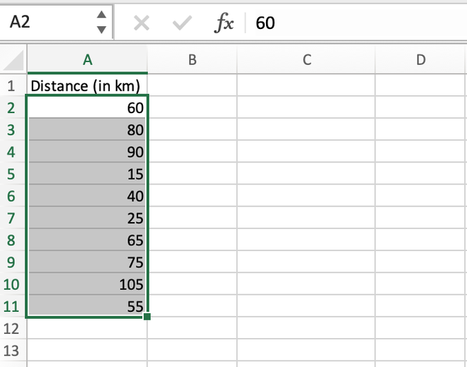
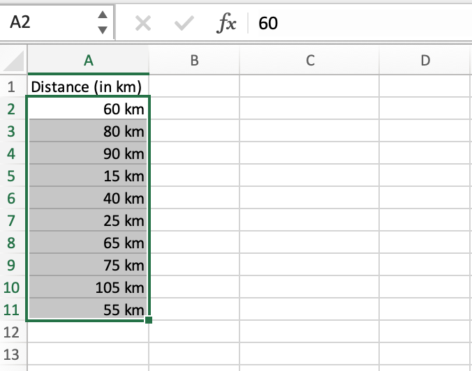
Step 1: Select the desired cells in which we want to apply the custom formatting.

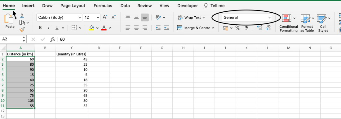
Step 2: In the topmost Excel ribbon, click on the Home tab and select the Number Format drop-down menu.

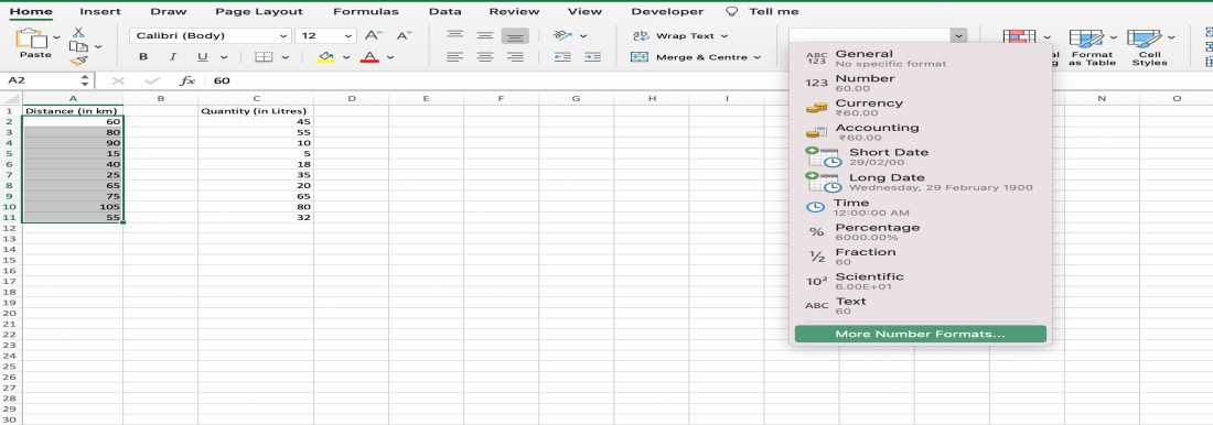
Step 3: In the drop-down list, select the More Number Format option to open the Format Cells dialog box.

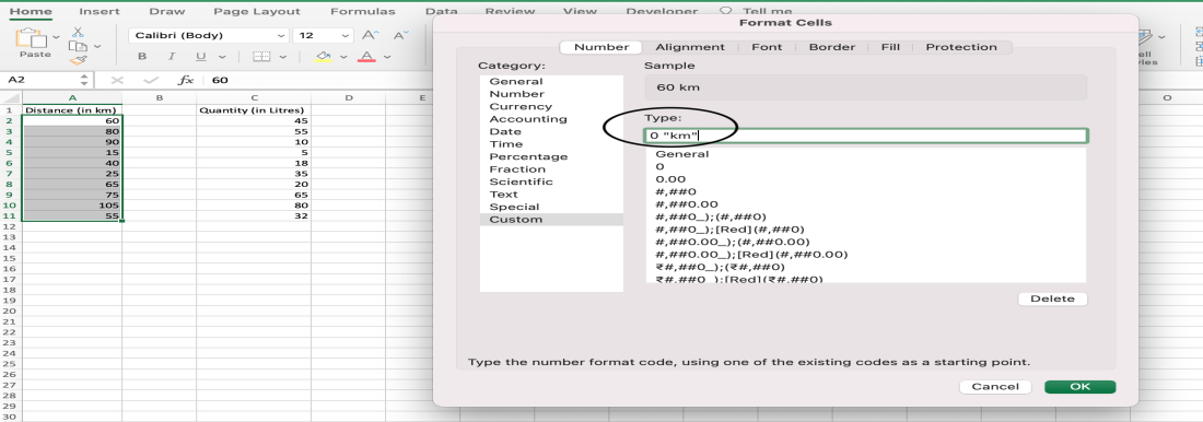
Step 4: In the Format Cells dialog box, on the left-hand side from the Category column select the Custom option.

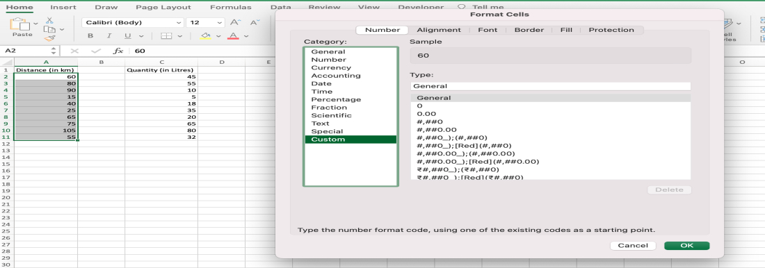
Step 5: From the built-in templates, select a matching number format code and then in the Type box inside double quotation marks (“”) write your desired unit, let’s say “Km.”.

Step 6: We can visualize what our data will look like after applying that formatting using the Sample tab.

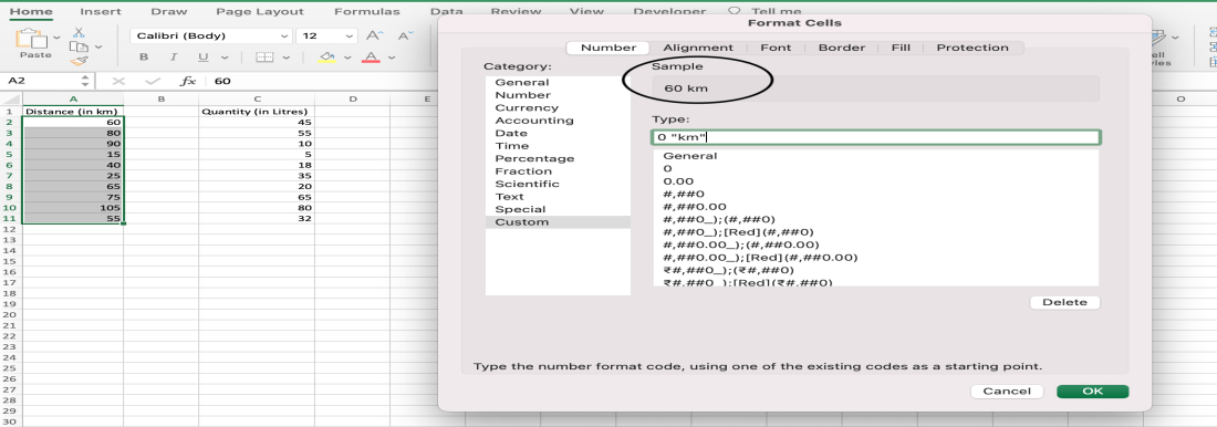
Step 7: After getting satisfied with the result we can click on the OK button to apply that formatting to all the desired cells.

Note: After selecting the desired cells, a user can directly open the Format Cells dialog box by using the “Ctrl + 1″ shortcut key on the keyboard in Windows OS or the “command + 1” shortcut key on macOS depending upon their operating system in which they are using Microsoft Excel. 

After applying custom formatting, we can even verify that our records are treated as numbers or not by applying any mathematical function like SUM() or AVERAGE(), these functions should be able to return the proper result which successfully demonstrates that our data records are still treated as numbers even after adding text to them.