Create Heatmap in R

Heatmap is a graphical way to represent data. It is most commonly used in data analysis. In data analysis, we explore the dataset and draws insight from the dataset, we try to find the hidden patterns in the data by doing a visual analysis of the data. Heatmap visualizes the value of the matrix with colours, where brighter the colour means the higher the value is, and lighter the colour means the lower the value is. In Heatmap, we use warmth to cool colour scheme. Heatmap is a so-called heatmap because in heatmap we map the colours onto the different values that we have in our dataset.

In this article, we will discuss how to create heatmaps in R Programming Language.

Method 1: Using the geom_tile() from the ggplot2 package

geom_tile() is used to create a 2-Dimensional heatmap with the plane rectangular tiles in it. It comes pre-installed with the ggplot2 package for R programming.

Syntax:

geom_tile( mapping =NULL, data=NULL, stat=”Identity”,…)

Parameter:

• mapping: It can be “aes”. “aes” is an acronym for aesthetic mapping. It describes how variables in the data are mapped to the visual properties of the geometry.
• data: It holds the dataset variable, a variable where we have stored our dataset in the script.
• stat: It is used to perform any kind of statistical operation on the dataset.

To create a heatmap, first, import the required libraries and then either create or load a dataset. Now simply call geom_tile() function with the appropriate values for parameters.

Example:

R

# Plotting Heatmap in R

# adding ggplot2 library for plotting
library(ggplot2)

# Creating random dataset
# with 20 alphabets and 20 animal names
letters <- LETTERS[1:20]
animal_names <- c("Canidae","Felidae","Cat","Cattle",
                  "Dog","Donkey","Goat","Guinea pig",
                  "Horse","Pig","Rabbit","Badger",
                  "Bald eagle","Bandicoot","Barnacle",
                  "Bass","Bat","Bear","Beaver","Bedbug",
                  "Bee","Beetle")

data <- expand.grid(X=letters, Y=animal_names)
data$count <- runif(440, 0, 6)

# plotting the heatmap
plt <- ggplot(data,aes( X, Y,fill=count))
plt <- plt + geom_tile()

# further customizing the heatmap by
# applying colors and title
plt <- plt + theme_minimal()

# setting gradient color as red and white
plt <- plt + scale_fill_gradient(low="white", high="red")

# setting the title and subtitles using
# title and subtitle
plt <- plt + labs(title = "Heatmap")
plt <- plt + labs(subtitle = "A simple heatmap using geom_tile()")

# setting x and y labels using labs
plt <- plt + labs(x ="Alphabets", y ="Random column names")

# plotting the Heatmap
plt

R

# Plotting Heatmap in R

# adding ggplot2 library for plotting
library(ggplot2)

# Creating random dataset
# with 20 alphabets and 20 animal names
letters <- LETTERS[1:20]
animal_names <- c("Canidae","Felidae","Cat","Cattle",
                  "Dog","Donkey","Goat","Guinea pig",
                  "Horse","Pig","Rabbit","Badger",
                  "Bald eagle","Bandicoot","Barnacle",
                  "Bass","Bat","Bear","Beaver","Bedbug",
                  "Bee","Beetle")

data <- expand.grid(X=letters, Y=animal_names)
data$count <- runif(440, 0, 6)

# plotting the heatmap
plt <- ggplot(data,aes( X, Y,fill=count))
plt <- plt + geom_tile()

# further customizing the heatmap by
# applying colors and title
plt <- plt + theme_minimal()

# setting gradient color as red and white
plt <- plt + scale_fill_gradient(low="white", high="red")

# setting the title and subtitles using
# title and subtitle
plt <- plt + labs(title = "Heatmap")
plt <- plt + labs(subtitle = "A simple heatmap using geom_tile()")

# setting x and y labels using labs
plt <- plt + labs(x ="Alphabets", y ="Random column names")

# plotting the Heatmap
plt

Output:

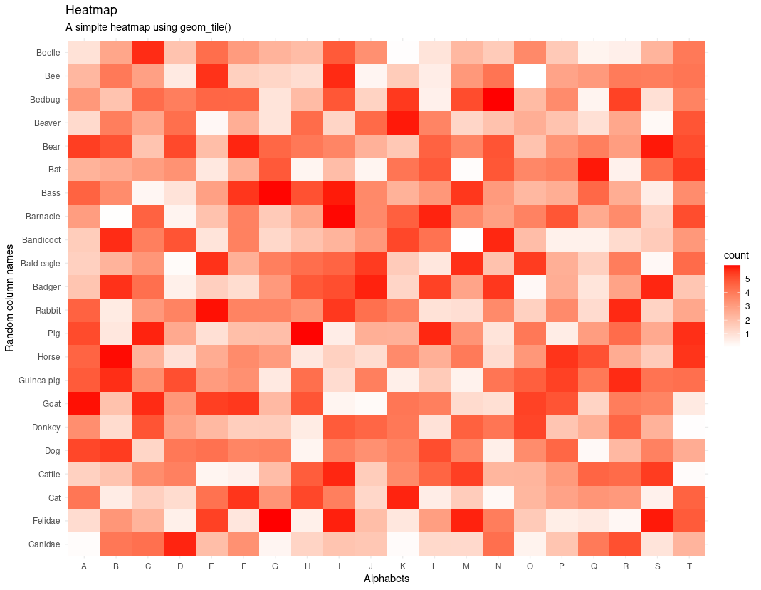
Heatmap using ggplot2

Method 2: Using heatmap() function of base R 

heatmap()  function comes with the default installation of the Base R. One can use the default heatmap() also if he does not want to install any extra package. We can plot heatmap of the dataset using this heatmap function from the R. 

Syntax:

heatmap(data,main = NULL, xlab = NULL, ylab = NULL,…)

Parameter:

data: data specifies the matrix of the data for which we wanted to plot a Heatmap.

main: main is a string argument, and it specifies the title of the plot.

xlab: xlab is used to specify the x-axis labels.

ylab: ylab is used to specify the y-axis labels.

Here the task is straightforward. You only need to put in the values that the function heatmap() requires.

Example:

R

# Heatplot from Base R
# using default mtcars dataset from the R
x  <- as.matrix(mtcars)

# custom colors
new_colors <- colorRampPalette(c("cyan", "darkgreen"))

# plotting the heatmap
plt <- heatmap(x,
               # assigning new colors
               col = new_colors(100),

               # adding title
               main = "Heatmap for mtcars dataset",

               # adding some margin so that
               # it does not drawn over the
               # y-axis label
               margins = c(5,10),

               # adding x-axis labels
               xlab = "variables",

               # adding y-axis labels
               ylab = "Car Models",

               # to scaled the values into
               # column direction
               scale = "column"
)

Output:

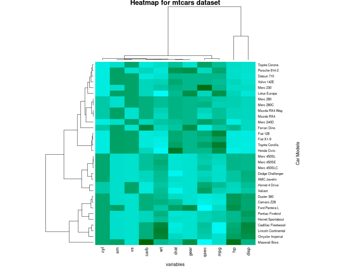
Heatmap