The COUNTIF function in Excel is used to count the number of cells that match a single condition applied. It can include Dates, Numbers, and Texts. It uses various logical operators like <(Less Than), >(Greater Than), >=(Greater Than or Equal to), <=(Less Than or Equal to), =(Equals to), and <>(NOT) for matching the condition. It also uses some wildcards like * and ? for partial matching.
How to Use Excel COUNTIF Function (with Examples)
COUNTIF Function is one of the Statistical Functions, to count the number of cells that meet a criterion; for example, to count the number of times a student appears in an attendance list.
The simplest form of COUNTIF is:
=COUNTIF(Where do you want to look?, What do you want to look for?)
The COUNTIF function in Excel is used to count the number of cells.
Syntax:
COUNTIF (range, criteria)
Arguments:
1. range:- Here range refers to the range of the cells for which you want the cell count for a specific condition.
2. criteria:- Here criteria refers to the condition for which you want the cell count.
Return Value:- COUNTIF function in excel returns an integer value of the number of cells which satisfy the given condition.
COUNTIF Formula for Text and Numbers (Exact Match)
The COUNTIF function formula that counts text values matching a specified criterion is:
Cells containing an exact string of text:= COUNTIF( D8:D17,” Mark”).
So, you enter:
- A range is the first parameter;
- A comma as the delimiter;
- A word or several words are enclosed in quotes as the criteria.
You can also use a reference to any cell containing that word or words and get absolutely the same results, such as =COUNTIF(D8:D17, D9)
Similarly, COUNTIF formulas work for numbers. The below formula perfectly counts cells with quantity 71 in Column E.
=COUNTIF(E8:E17, 71)
.png)
COUNTIF Formulas with Wildcard Characters (partial match)
If your Excel data include several variations of the keywords you want to count, then you can use a Wildcard Character to count the cells containing that particular word, phrase, or letter as a cell’s content.
For example, you have a list of students with their marks and we want to know how many marks Rocky Sharma got. But his name is written in several different ways, we enter “*Sharma*” as the search criteria =COUNTIF( B22:B28,”*Sharma*”)
.png)
Note: An asterisk (*) is used to find cells with any sequence of leading or trailing characters, as illustrated in the above example. You have to enter a question mark (?) to match any single character.
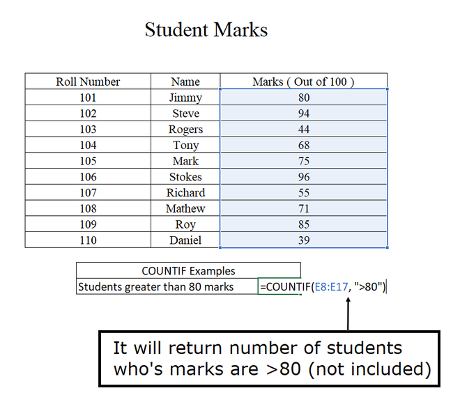
COUNTIF Greater than, Less than, or Equal to
To count cells with values greater than, less than, or equal to the number you specify, you simply add a corresponding operator to the criteria.
Consider the student’s marks which are given below for and XYZ examination.
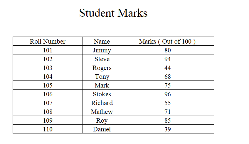
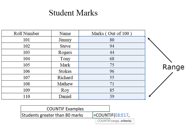
Understanding the arguments of the COUNTIF function in Excel
Understanding the argument of the COUNTIF function in Excel
Output:
Note: RED color cells are used for the reference that which cells would satisfy the given criteria. RED color doesn’t come in the output of COUNTIF.
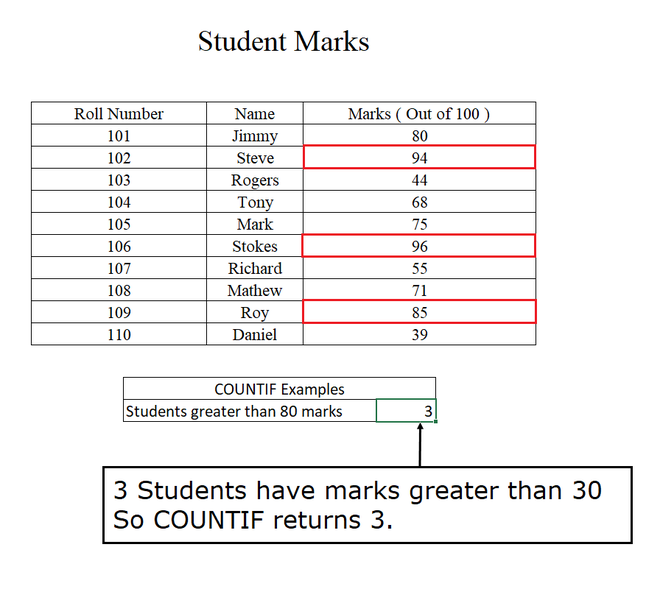
The output of the marks of the students having greater than 80
Example 2:
COUNTIF Not Blank
This formula example demonstrates how you use the COUNTIF function in Excel to count the number of blank cells in a specified range.
=COUNTIF( C1:C10,”*”)
But the problem with this formula is that it counts only cells containing any text values including empty strings, which means cells with dates and numbers will be treated as blank cells and not be included in the count.
Below is the universal COUNTIF formula for counting all non-blanks cells in a specified range:
COUNTIF(range, “<>”)
Or
COUNTIF (range,”<>”&””)
The above formula works well with all value types -text, dates, and numbers.
COUNTIF Blank
If you want to count blank cells in a certain range, use the formula with a wildcard character for text values and with the “” criteria to count all empty cells.
Formula to count blank cells:
COUNTIF(range,”<>”&”*”)
Note: Asterisk(*) is used because it matches any sequence of text characters, the formula counts cells not equal to *, which doesn’t contains any text in the specified range
COUNTIF formula for blanks (all value types):
COUNTIF(range,” “)
.png)
Excel COUNTIF with dates
If you want to Count cells with dates that are greater than, less than, or equal to the date you specify in another cell. All the above-discussed formulas work for dates as well as numbers.
Below are some examples to count the cells which have dates in them with different formats.
|
Count dates equal to the specified date.
|
=COUNTIF(A2:A10,”6/1/2014″)
|
Counts the number of cells in the range A2:A10 with the date 1-jun-2014
|
| Count dates greater than or equal to another date. |
=COUNTIF(A2:A10,”>=6/1/2014) |
Count the number of cells in the range A2:A10 with a date greater than or equal to 6/1/2014. |
|
Count dates greater than or equal to a date in another cell, Minus x days.
|
=COUNTIF(A2:A10,”>=”&A2-“7”)
|
Count the number of cells in the range A2:A10 with a date greater than or equal to the date in A2 minus 7 days.
|
Apart from this, you can use the COUNTIF function in conjunction with specific Excel Date and Time functions such as TODAY() to count cells based on the current date.
|
Count dates equal to the current date.
|
=COUNTIF(A2:A10,TODAY())
|
|
Count dates prior to the current date,i.e. less than today.
|
=COUNTIF(A2:A10,”<“&TODAY())
|
|
Count dates after the current date, i.e. greater than today.
|
=COUNTIF(A2:A10,”>”&TODAY())
|
|
Count dates that are due in a week.
|
=COUNTIF(A2:A10,”=”&TODAY()+7)
|
|
Count dates in a specific range.
|
=COUNTIF(B2:B10,”>=6/1/2023″)- COUNTIF(B2:B10,”>6/7/2023″)
|
Excel COUNTIF with Multiple Criteria
COUNTIF Function is not exactly designed to count cells with multiple criteria. The COUNTIFS function is used to count cells that match two or more criteria(AND logic). You can combine two or more COUNTIF functions in one formula to solve some easy tasks.
Count Values between two numbers
The most common application of Excel COUNTIF function with 2 criteria is counting numbers within a specific range, i.e. less than X but greater than Y.
Below is a formula that is used to count cells in the range A2:A9 where a value is greater than 5 and less than 15.
=COUNTIF(A2:A9,”>5″)- COUNTIF(A2:A9,”=15)
.png)
Using the COUNTIF Function to find Duplicates and Unique Values
We can also use the COUNTIF function for finding duplicates in one column, between two columns, or in a row.
Example 1: Find and count duplicates in 1 column
The formula =COUNTIF(A2:A10, A2)>1 will spot all duplicate entries in the range A2:A10 while another function =COUNTIF(B2:B10, TRUE) will tell you how many duplicates are there
Example 2: Count duplicates between two columns
Suppose you have two separate lists, say lists of names in columns B and C, and you want to find out how many appear in both columns, you can use Excel COUNTIF in combination with the SUMPRODUCT function to count duplicates.
=SUMPRODUCT0((COUNTIF(B2:B1000,C2:C1000)>0)*(C2:C1000<>””))
To count how many unique names are there in Column C, i.e. names that do NOT appear in Column B:
=SUMPRODUCT((COUNTIF(A2:A1000,C2:C1000)=0)*(C2:C1000<>””))
Example 3: Count duplicates and unique values in a row
You can use one of the below formulae to count duplicates or unique values in a certain row rather than a column.
Count duplicates in a row:
=SUMPRODUCT ((COUNTIF(A5:J5,A5:J5)>1)*(A5:J5<>” “))
Count unique values in a row:
=SUMPRODUCT((COUNTIF(A5:J5,A5:J5)=1*(A5:J5<>” “))
Important Points to remember
- COUNTIF is not case-sensitive.
- COUNTIF will only check one condition at a time.
- COUNTIF needs a range for the evaluation.
- In COUNTIF the criteria must be enclosed in the double-quotes.
- If the criteria are evaluated from a different cell then that cell must not be enclosed in the double-quotes. E.g. “=” & E5
- It gives an error if the matching string exceeds 255 characters.
FAQs
What is the COUNTIF function in Excel?
The COUNTIF function in Excel is used to count the number of cells that match a single condition applied. It can include Dates, Numbers, and Texts. It uses various logical operators like <(Less Than), >(Greater Than), >=(Greater Than or Equal to), <=(Less Than or Equal to), =(Equals to), and <>(NOT) for matching the condition. It also uses some wildcards like * and ? for partial matching.
When to use an ampersand in a COUNTIF formula?
If you use a number or a cell reference in the exact match criteria, you need neither ampersand nor quotes. For example
=COUNTIF(A2:A10,100) Or
=COUNTIF(A2:A10,D2)
If your criteria is an expression with a cell reference or another Excel function, you have to use quotes(“”) to start the text string and ampersand (&) to concatenate and finish the string off For example :
=COUNTIF(A2:A10,”>”&D2) Or
=COUNTIF(A2:A10,”<=”&Today())
How can we use COUNTIF in Excel on a non-contiguous range or a selection of cells?
Excel doesn’t work on non- adjacent range, nor does its syntax allow specifying several individual cells as the first parameter.
You can use a combination of several COUNTIF functions:
=COUNTIF(A2,”>0″) + COUNTIF(B3,”>)”) + COUNTIF (C4,”>0″)
Like Article
Suggest improvement
Share your thoughts in the comments
Please Login to comment...