Correlation Matrix in R Programming

Correlation refers to the relationship between two variables. It refers to the degree of linear correlation between any two random variables. This Correlation Matrix in R can be expressed as a range of values expressed within the interval [-1, 1]. The value -1 indicates a perfect non-linear (negative) relationship, 1 is a perfect positive linear relationship and 0 is an intermediate between neither positive nor negative linear interdependency. Hoindependent of each other completely. Correlation Matrix in R computes the linear relationship degree between a set of random variables, taking one pair at a time and performing for each set of pairs within the data.

Properties of Correlation Matrix in R

• All the diagonal elements of the Correlation Matrix in R must be 1 because the correlation of a variable with itself is always perfect, c_ii=1.
• It should be symmetric c_ij=c_ji.

Computing Correlation Matrix in R

In R Programming Language, a correlation matrix can be completed using the cor( ) function, which has the following syntax:

 Syntax: cor (x, use = , method =    )

Parameters:

x: It is a numeric matrix or a data frame.
use: Deals with missing data.

• all.obs: this parameter value assumes that the data frame has no missing values and throws an error in case of violation.
• complete.obs: listwise deletion.
• pairwise.complete.obs: pairwise deletion.

method: Deals with a type of relationship. Either Pearson, Spearman, or Kendall can be used for computation. The default method used is Pearson. 

Correlation in R Programming Language

The Correlation Matrix in R is done after loading the data. The following code snippet indicates the usage of the cor() function: 

R

# loading dataset from the specified url
# storing the data into csv
data = read.csv("https://people.sc.fsu.edu/~jburkardt/data/csv/ford_escort.csv",
                header = TRUE, fileEncoding = "latin1")

# printing the head of the data
print ("Original Data")
head(data)

# computing correlation matrix
cor_data = cor(data)

print("Correlation matrix")
print(cor_data)

Output:

[1] "Original Data"
  Year Mileage..thousands. Price
1 1998                  27  9991
2 1997                  17  9925
3 1998                  28 10491
4 1998                   5 10990
5 1997                  38  9493
6 1997                  36  9991
[1] "Correlation matrix"
                         Year Mileage..thousands.      Price
Year                 1.0000000          -0.7480982  0.9343679
Mileage..thousands. -0.7480982           1.0000000 -0.8113807
Price                0.9343679          -0.8113807  1.0000000

Computing Correlation Coefficients of Correlation Matrix in R

R contains an in-built function rcorr() which generates the correlation coefficients and a table of p-values for all possible column pairs of a data frame. This function basically computes the significance levels for Pearson and spearman correlations.

Syntax: rcorr (x, type = c(“pearson”, “spearman”))

In order to run this function in R, we need to download and load the “Hmisc” package into the environment. This can be done in the following way: 

install.packages(“Hmisc”) 

library(“Hmisc”)

The following code snippet indicates the computation of correlation coefficients in R:

R

data = read.csv("https://people.sc.fsu.edu/~jburkardt/data/csv/ford_escort.csv",
                header = TRUE, fileEncoding = "latin1")

# printing the head of the data
print("Original Data")
head(data)

# installing the library of Hmisc
install.packages("Hmisc")
library("Hmisc")

# computing p values of the data loaded
p_values <- rcorr(as.matrix(data))
print(p_values)

Output:

[1] "Original Data"
Year Mileage..thousands. Price
1 1998                  27  9991
2 1997                  17  9925
3 1998                  28 10491
4 1998                   5 10990
5 1997                  38  9493
6 1997                  36  9991
Year Mileage..thousands. Price
Year                 1.00               -0.75  0.93
Mileage..thousands. -0.75                1.00 -0.81
Price                0.93               -0.81  1.00
n= 23 
P
                    Year Mileage..thousands. Price
Year                      0                   0   
Mileage..thousands.  0                        0   
Price                0    0                       

Visualize a Correlation Matrix in R

In R, we shall use the “corrplot” package to implement a correlogram. Hence, to install the package from the R Console we should execute the following command:

install.packages("corrplot")

Once we have installed the package properly, we shall load the package in our R script using the library() function as follows:  

library("corrplot")

We will use the corrplot() function and mention the shape in its method arguments.

R

# Correlogram in R
# required packages
library(corrplot)

head(mtcars)
# correlation matrix
M<-cor(mtcars)
head(round(M,2))

# visualizing correlogram
# as circle
corrplot(M, method="circle")

# as pie
corrplot(M, method="pie")

# as colour
corrplot(M, method="color")

# as number
corrplot(M, method="number")

Output:

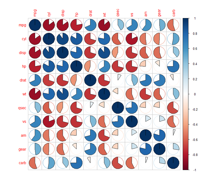
Visualize Correlogram as a pie chart

R

# as pie
corrplot(M, method="pie")

Output:

Visualize Correlogram as colored rectangles

R

# as colour
corrplot(M, method="color")

Output:

Visualize Correlogram as numbers

R

# Correlogram as numbers
corrplot(M, method="number")

Output:

Visualize Correlogram as 3D Scatter Plot

R

corrplot(correlation_matrix, method="ellipse")

Output:

Correlation Matrix in R Programming

Visualize Correlogram as Density Plot

R

corrplot(M, method="shade")

Output:

Correlation Matrix in R Programming

We can choose the visualization method that best suits your needs or preferences. The corrplot package provides various customization options for each visualization method.