Convolution Theorem for Fourier Transform MATLAB

A Convolution Theorem states that convolution in the spatial domain is equal to the inverse Fourier transformation of the pointwise multiplication of both Fourier transformed signal and Fourier transformed padded filter (to the same size as that of the signal). In other words, the convolution theorem says that Convolution in the spatial domain can be carried out in the frequency domain using Fourier transformation.

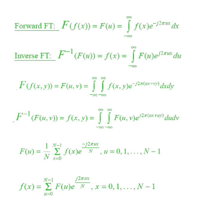
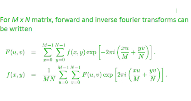
Equation for Discrete Fourier Transformation (DFT):

Equation for Inverse DFT:

Steps:

• We have image M and spatial filter S.
• Since we need pointwise multiplication, filter size should be equal to image size.
• Pad the filter S with 0’s to make its size equal to image M. Padded filter S’.
• Take Fourier Transformation of both M and S’.
• Take pointwise multiplication of FT(M) and FT(S’)
• Take inverse Fourier Transformation of the result.

Function Used:

• imread( ) inbuilt function is used to read the image.
• size( ) inbuilt function is used to get size of image.
• rgb2gray( ) inbuilt function is used to convert RGB image into grayscale image.
• ones( ) inbuilt function is used to create matrix of 1s.
• conv2( ) inbuilt function is used to perform 2D convolution.
• imtool( ) inbuilt function is used to display images.
• fft2( ) inbuilt function is used to perform 2D Fourier Transformation.
• ifft2( ) inbuilt function is used to perform inverse 2D Fourier Transformation.
• fftshift( ) inbuilt function is used to shift corners of FT into center.
• pause( ) inbuilt function is used to pause the execution for specified seconds.

Example:

Matlab

% MATLAB code for Convolution in Spatial Domain:
% CONVOLUTION IN SPATIAL DOMAIN
function f=Convolution(img)

%convert into grayscale if not.
[x,y,z]=size(img);
if(z==3)
    img=rgb2gray(img);
end

% Define averaging filter
mask=ones(5,5).*1/25;
Original_input_image=double(img);
convolved_image=conv2(Original_input_image,mask,'same');

% Display images.
imtool(Original_input_image,[]);
imtool(convolved_image,[]);

% Close all image tabs after 10s.
pause(10);
imtool close all;
end

% Utility code
k=imread("cameraman.jpg");
Convolution(k);

Output:

Code Explanation:

• mask=ones(5,5).*1/25; This line creates the averaging filter of size [5 5]
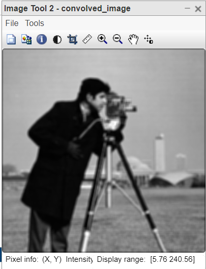
• convolved_image=conv2(Original_input_image,mask,’same’); This line performs the convolution between image and filter.
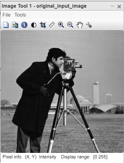
• imtool(Original_input_image,[]); This line displays input image.
• imtool(convolved_image,[]); This line displays convolved imaged.
• pause(10); This line has the execution for 10 seconds.
• imtool close all; This line closes all images windows.
• k=imread(“cameraman.jpg”); This line reads the image.
• Convolution(k); This line calls the function by passing the image as a parameter.

Example:

Matlab

% MATLAB code for Convolution in Frequency Domain:
% CONVOLUTION THEOREM FOR FOURIER TRANSFORMATION
function f=Convolution_Theorem(img)

% Convert into grayscale if not.
[x,y,z]=size(img);
if(z==3)
    img=rgb2gray(img);
end

% Define averaging filter
mask=ones(5,5).*1/25;
FT_img=fft2(img);
FT_mask=fft2(mask,x,y);

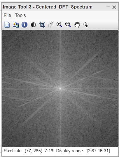
Fourier_Transformed_image=abs(log(fftshift(FT_img)));
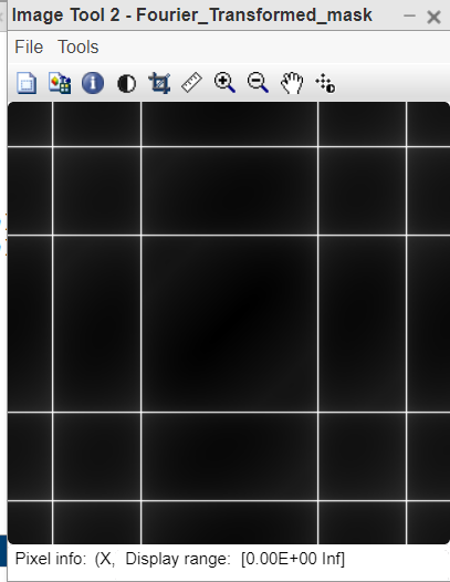
Fourier_Transformed_mask=abs(log(fftshift(FT_mask)));
imtool(Fourier_Transformed_image,[]);
imtool(Fourier_Transformed_mask,[]);

pointwise_mul=FT_img.*FT_mask;
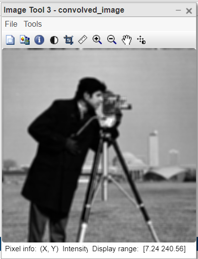
convolved_image=ifft2(pointwise_mul);
imtool(convolved_image,[]);

% Close all image tabs after 15s.
pause(15);
imtool close all;
end

% UTILITY CODE
k=imread("cameraman.jpg");
Convolution_Theorem(k);

Output:

Code Explanation:

• mask=ones(5,5).*1/25; This line creates the averaging filter of size [5 5].
• FT_img=fft2(img); This line computes the FT of input image.
• FT_mask=fft2(mask,x,y); This line computes the FT of the averaging mask created above.
• pointwise_mul=FT_img.*FT_mask; This line performs the element-wise multiplication between FT image and mask.
• convolved_image=ifft2(pointwise_mul); This line applies inverse shifting: image quadrants are exchanged diagonally.
• k=imread(“cameraman.jpg”); This line reads the image.
• Convolution_Theorem(k); This line passes the input image to the function.

Fourier transformation is faster than convolution in the spatial domain. Computation complexity is less in the frequency domain. In MATLAB the inbuilt function “conv2” also uses the same technique to perform convolution. The image and the mask are converted into the frequency domain, by using Fourier Transformation. The inverse FT is performed on the pointwise multiplication of image and mask. 

If we perform the convolution as per the mathematics in the spatial domain, it would take more time as it includes more computation. If the filter size is small and the matrix is large then computational cost increase significantly.