Contractive Autoencoder (CAE)
Last Updated :
20 Mar, 2024
In this article, we will learn about Contractive Autoencoders which come in very handy while extracting features from the images, and how normal autoencoders have been improved to create Contractive Autoencoders.
What is Contarctive AutoEncoder?
Contractive Autoencoder was proposed by researchers at the University of Toronto in 2011 in the paper Contractive auto-encoders: Explicit invariance during feature extraction. The idea behind that is to make the autoencoders robust to small changes in the training dataset.
To deal with the above challenge that is posed by basic autoencoders, the authors proposed adding another penalty term to the loss function of autoencoders. We will discuss this loss function in detail.
Loss Function of Contactive AutoEncoder
Contractive autoencoder adds an extra term in the loss function of autoencoder, it is given as:

i.e. the above penalty term is the Frobenius Norm of the encoder, the Frobenius norm is just a generalization of the Euclidean norm.
In the above penalty term, we first need to calculate the Jacobian matrix of the hidden layer, calculating a Jacobian of the hidden layer with respect to input is similar to gradient calculation. Let’s first calculate the Jacobian of the hidden layer:

where \phi is non-linearity. Now, to get the jth hidden unit, we need to get the dot product of the ith feature vector and the corresponding weight. For this, we need to apply the chain rule.
![\begin{aligned} \frac{\partial h_j}{\partial X_i} &= \frac{\partial \phi(Z_j)}{\partial X_i} \\ &= \frac{\partial \phi(W_i X_i)}{\partial W_i X_i} \frac{\partial W_i X_i}{\partial X_i} \\ &= [\phi(W_i X_i)(1 - \phi(W_i X_i))] \, W_{i} \\ &= [h_j(1 - h_j)] \, W_i \end{aligned}](https://quicklatex.com/cache3/a9/ql_e9fe96182e289452c76e30bb8f6dcfa9_l3.png "Rendered by QuickLaTeX.com")
The above method is similar to how we calculate the gradient descent, but there is one major difference, that is we take h(X) as a vector-valued function, each as a separate output. Intuitively, For example, we have 64 hidden units, then we have 64 function outputs, and so we will have a gradient vector for each of that 64 hidden units.
Let diag(x) be the diagonal matrix, the matrix from the above derivative is as follows:
![\frac{\partial h}{\partial X} = diag[h(1 - h)] \, W^T](https://www.geeksforgeeks.org/wp-content/ql-cache/quicklatex.com-685c0baf8566c3f6c7c7999055b0527e_l3.png "Rendered by QuickLaTeX.com")
Now, we place the diag(x) equation to the above equation and simplify:
![\begin{aligned}\lVert J_h(X) \rVert_F^2 &= \sum_{ij} \left( \frac{\partial h_j}{\partial X_i} \right)^2 \\[10pt] &= \sum_i \sum_j [h_j(1 - h_j)]^2 (W_{ji}^T)^2 \\[10pt] &= \sum_j [h_j(1 - h_j)]^2 \sum_i (W_{ji}^T)^2 \\[10pt]\end{aligned}](https://quicklatex.com/cache3/76/ql_e88ebf31f5ebe3e56afa70f6e3b3c976_l3.png "Rendered by QuickLaTeX.com")
Relationship with Sparse Autoencoder
In sparse autoencoder, our goal is to have the majority of components of representation close to 0, for this to happen, they must be lying in the left saturated part of the sigmoid function, where their corresponding sigmoid value is close to 0 with a very small first derivative, which in turn leads to the very small entries in the Jacobian matrix. This leads to highly contractive mapping in the sparse autoencoder, even though this is not the goal in sparse Autoencoder.
Relationship with Denoising Autoencoder
The idea behind denoising autoencoder is just to increase the robustness of the encoder to the small changes in the training data which is quite similar to the motivation of Contractive Autoencoder. However, there is some difference:
- CAEs encourage robustness of representation f(x), whereas DAEs encourage robustness of reconstruction, which only partially increases the robustness of representation.
- DAE increases its robustness by stochastically training the model for the reconstruction, whereas CAE increases the robustness of the first derivative of the Jacobian matrix.
Contractive Autoencoder (CAE) Implementation Stepwise
Import the TensorFlow and load the dataset
Python3
import tensorflow as tf

# load dataset
(x_train, _), (x_test, _) = tf.keras.datasets.fashion_mnist.load_data()
x_train = x_train.astype('float32') / 255.
x_test = x_test.astype('float32') / 255.
Build the Contractive Autoencoder (CAE) Model
Python3
class AutoEncoder(tf.keras.Model):
    def __init__(self):
        super(AutoEncoder, self).__init__()
        self.flatten_layer  =tf.keras.layers.Flatten()
        self.dense1 = tf.keras.layers.Dense(64, activation=tf.nn.relu)
        self.dense2 = tf.keras.layers.Dense(32, activation=tf.nn.relu)


        self.bottleneck = tf.keras.layers.Dense(16, activation=tf.nn.relu)

        self.dense4 = tf.keras.layers.Dense(32, activation=tf.nn.relu)
        self.dense5 = tf.keras.layers.Dense(64, activation=tf.nn.relu)

        self.dense_final = tf.keras.layers.Dense(784)

    def call(self, inp):
        x_reshaped = self.flatten_layer(inp)
        #print(x_reshaped.shape)
        x = self.dense1(x_reshaped)
        x = self.dense2(x)
        x = self.bottleneck(x)
        x_hid= x
        x = self.dense4(x)
        x = self.dense5(x)
        x = self.dense_final(x)
        return x, x_reshaped,x_hid
Define the loss function
Python3
# define loss function and gradient
def loss(x, x_bar, h, model, Lambda =100):
    reconstruction_loss = tf.reduce_mean(
                tf.keras.losses.mse(x, x_bar)
            )
    reconstruction_loss *= 28 * 28
    W= tf.Variable(model.bottleneck.weights[0])
    dh = h * (1 - h)  # N_batch x N_hidden
    W = tf.transpose(W)
    contractive = Lambda * tf.reduce_sum(tf.linalg.matmul(dh**2,
                                                          tf.square(W)),
                                         axis=1)
    total_loss = reconstruction_loss + contractive
    return total_loss
Define the Gradient
Python3
def grad(model, inputs):
    with tf.GradientTape() as tape:
        reconstruction, inputs_reshaped, hidden = model(inputs)
        loss_value = loss(inputs_reshaped, reconstruction, hidden, model)
    return loss_value, tape.gradient(loss_value, model.trainable_variables), inputs_reshaped, reconstruction
Train the model
Python3
# train the model
model = AutoEncoder()
optimizer = tf.optimizers.Adam(learning_rate=0.001)
global_step = tf.Variable(0)
num_epochs = 200
batch_size = 128
for epoch in range(num_epochs):
    print("Epoch: ", epoch)
    for x in range(0, len(x_train), batch_size):
        x_inp = x_train[x : x + batch_size]
        loss_value, grads, inputs_reshaped, reconstruction = grad(model, x_inp)
        optimizer.apply_gradients(zip(grads, model.trainable_variables),
                              global_step)

    print("Step: {}, Loss: {}".format(global_step.numpy(),tf.reduce_sum(loss_value)))
Output:
Epoch:  0
Step: 0, Loss: 3717.4609375
Epoch:  1
Step: 0, Loss: 3014.34912109375
Epoch:  2
Step: 0, Loss: 2702.09765625
Epoch:  3
Step: 0, Loss: 2597.461669921875
Epoch:  4
Step: 0, Loss: 2489.85693359375
Epoch:  5
Step: 0, Loss: 2351.0146484375
Epoch:  6
Step: 0, Loss: 2094.60693359375
Epoch:  7
Step: 0, Loss: 1996.68994140625
Epoch:  8
Step: 0, Loss: 1930.5377197265625
Epoch:  9
Step: 0, Loss: 1881.977294921875
...
...
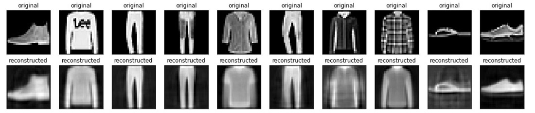
Generate results
Python3
# generate results
n = 10
import matplotlib.pyplot as plt
plt.figure(figsize=(20, 4))
for i in range(n):
  # display original
  ax = plt.subplot(2, n, i + 1)
  plt.imshow(x_test[i])
  plt.title("original")
  plt.gray()
  ax.get_xaxis().set_visible(False)
  ax.get_yaxis().set_visible(False)

  # display reconstruction
  ax = plt.subplot(2, n, i + 1 + n)
  reconstruction, inputs_reshaped,hidden = model(x_test[i].reshape((1,784)))
  plt.imshow(reconstruction.numpy().reshape((28,28)))
  plt.title("reconstructed")
  plt.gray()
  ax.get_xaxis().set_visible(False)
  ax.get_yaxis().set_visible(False)
plt.show()
Output:
Like Article
Suggest improvement
Share your thoughts in the comments
Please Login to comment...