Constraint Cubic spline
Last Updated :
24 Oct, 2021
Cubic Spline Interpolation
Cubic spline interpolation is a way of finding a curve that connects data points with a degree of three or less. Splines are polynomial that are smooth and continuous across a given plot and also continuous first and second derivatives where they join.
We take a set of points [xi, yi] for i = 0, 1, …, n for the function y = f(x). The cubic spline interpolation is a piecewise continuous curve, passing through each of the values in the table.
- Following are the conditions for the spline of degree K=3:
- The domain of s is in intervals of [a, b].
- S, S’, S” are all continuous function on [a,b].
![S(x) =\begin{bmatrix} S_0 (x), x \epsilon [x_0, x_1] \\ S_1 (x), x \epsilon [x_1, x_2] \\ ... \\ ... \\ ... \\ S_{n-1} (x), x \epsilon [x_1, x_2] \end{bmatrix}](https://www.geeksforgeeks.org/wp-content/ql-cache/quicklatex.com-bfe0b4a8fddd8d349888f0eb303f7f44_l3.png "Rendered by QuickLaTeX.com")
Here Si(x) is the cubic polynomial that will be used on the subinterval [xi, xi+1].
The main factor about spline is that it combines different polynomials and does not use a single polynomial of degree n to fit all the points at once, it avoids high degree polynomials and thereby the potential problem of overfitting. These low-degree polynomials need to be such that the spline they form is not only continuous but also smooth.
But for the spline to be smooth and continuous, the two consecutive polynomials and Si (x) and Si+1 (x) must join at xi.

Or, Si (x) must be passed through two end-points:

Assume, S” (x) = Mi (i= 0,1,2, … , n). Since S(x) is cubic polynomial , so S” (x) is the linear polynomial in [xi, xi+1], then S”’ (x) will be:
![S''' (x) = \frac{M_{i+1} - M_i }{x_{i+1} - x_i} \, \forall x \epsilon [x_i, x_{i+1}]](https://www.geeksforgeeks.org/wp-content/ql-cache/quicklatex.com-1c32505b7ac87f0da679b14a1c63f3ae_l3.png "Rendered by QuickLaTeX.com")
By applying the Taylor series:

Let, x = xi+1:

Similarly, we apply above equation b/w range [xi-1, xi]:

Let hi =xi – xi-1

Now, we have n-1 equations, but have n+1 variables i.e M0, M1, M2,…Mn-1, Mn. Therefore, we need to get 2 more equations. For that, we will be using additional boundary conditions.
Let’s consider that we know S’ (x0) = f0‘ and S’ (xn) = fn‘, especially if S’ (x0) and S’ (xn) both are 0. This is called the clamped boundary condition.

![f_{0}^{'} = - M_0 \frac{h}{2} + f[x_0, x_1] - \frac{M_1 - M_0}{6}h_1](https://www.geeksforgeeks.org/wp-content/ql-cache/quicklatex.com-705d8826de69074b5b2b908881ab17fd_l3.png "Rendered by QuickLaTeX.com")
![2M_0 + M_1 = \frac{6}{h_1} (f[x_0, x_1] - f_{0}')](https://www.geeksforgeeks.org/wp-content/ql-cache/quicklatex.com-77dbad75e78cc4a7a6b6f70976ea7ce9_l3.png "Rendered by QuickLaTeX.com")
Similarly, for Mn
![2M_{n} + M_{n-1} = \frac{6}{h_n} (f_{n}' -f[x_{n-1}, x_n] )](https://www.geeksforgeeks.org/wp-content/ql-cache/quicklatex.com-14f8cfc70273796d25bf3d741add7386_l3.png "Rendered by QuickLaTeX.com")
or
![2M_{n} + M_{n-1} = {6}f[x_0, x_0, x_1] \\ d_n = f[x_{n-1}, x_n, x_n]](https://www.geeksforgeeks.org/wp-content/ql-cache/quicklatex.com-b444ad87090e51a4b1236bc283d364f2_l3.png "Rendered by QuickLaTeX.com")
Combining the above equation in to the matrix form, we get the following matrix:

Constraint Cubic Spline
Constraint cubic spline was proposed by the CJC Kruger in his article. The algorithm is an extension of cubic spline interpolation. The important step in it is the calculation of the slope at each point. The idea behind the slope calculation is that the slope at a point will be b/w the slope of the two adjacent lines joining that point, if one of them is 0 then the slope at point should also be 0.
Let take a collection of point (x_0, y_0), (x_1, x_2) …\, …\, … \, (x_{i-1}, y_{i-1}),(x_{i}, y_{i}), (x_{i+1}, y_{i+1})…\, …\, … \, (x_n, y_n). The cubic curve can be given by:

The above curve pass through all of the following points:

THe first order derivative must be continuous at intermediate points:

which can be calculated by following formula for intermediate points:
 if slope changes sign at point.
First derivative (slope) of each end point is calculated by following formula:

Second derivative are calculated by following formula:
![f_i^{''}(x_{i-1}) = \frac{2 [f_i^{'}(x_{i}) + 2f_i^{'}(x_{i-1}) ]}{x_i - x_{i-1}} + \frac{6(y_i - y_{i-1})}{(x_i - x_{i-1})^2} \\ f_i^{''}(x_{i}) = \frac{2 [2f_i^{'}(x_{i}) + f_i^{'}(x_{i-1}) ]}{x_i - x_{i-1}} - \frac{6(y_i - y_{i-1})}{(x_i - x_{i-1})^2}](https://www.geeksforgeeks.org/wp-content/ql-cache/quicklatex.com-5131cb275c8aa2abfeda6eb8fc718dcd_l3.png "Rendered by QuickLaTeX.com")
Solving for the coefficient of curve gives:

Conclusion
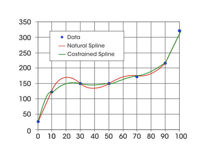
Constraint vs Natural Spline (Upward)
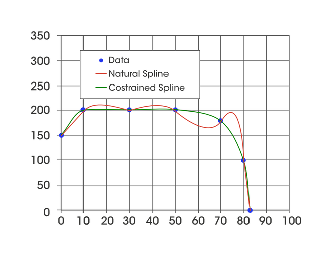
Constraint vs Cubic (downward)
Constraint cubic spline interpolation has the following advantages as compared to a standard cubic spline.
- It generates a relatively smooth curve as compare to standard cubic spline
- Interpolated values are calculated without solving a system of equations.
- It never overshoots the immediate values.
References:
Like Article
Suggest improvement
Share your thoughts in the comments
Please Login to comment...