Computer Graphics – 3D Composite Transformation

3-D Transformation is the process of manipulating the view of a three-D object with respect to its original position by modifying its physical attributes through various methods of transformation like Translation, Scaling, Rotation, Shear, etc.

Types of Transformation:

1. Translation Transformation
2. Scaling Transformation
3. Rotation Transformation
4. Shearing Transformation
5. Reflection Transformation

Note: If we’re asked to perform three or more different sorts of transformations over a point(P₀) simultaneously which is placed in 3D space, and let us assume that these transformations are T₁, T₂, and T₃ respectively, then in this case what we’ll do? 

So, we will see the following solutions

a) Obviously, first by applying series of Transformations one by one over the coordinates of the object sequentially.

First we performed transformation T_1, then P_o become transformed to P_1.

Secondly, we perform transformation T₂ and the point P₁ become transformed to P_2.

Lastly, we perform transformation T₃ and we get the final result i.e; P_3,and we will get our final transformed point coordinate(P₃).

b) Second solution, by applying Composite transformation in a single shot.

Note: Here T₁, T₂, T₃ correspond to their transformation matrix condition.

Composite Transformation

As its name suggests itself composite, here we compose two or more than two transformations together and calculate a resultant(R) transformation matrix by multiplying all the corresponding transformation matrix conditions with each other. 

The same equivalent result that we got over Point P₀ and transformed it into P₃ in the above example can also be achieved by directly multiplying resultant R with the point P₀ rather than performing transformations T₁, T₂, and T₃ sequentially one after one.

And we end up with the same equivalent result that we got into our above example.

Problem: Consider we are given with a cuboid “OABCDEFG” over which we want to perform 

• Translation transformation(T₁) if translation distances are D_x=2, D_y=3, D_z=2 ,then
• Scaling transformation(T₂) if scaling factors are s_x=2, s_y=1, s_z=3 and lastly perform,
• Shearing transformation(T₃) in x-direction if shearing factors are s_y=2 and s_z=1.

Solution: We are given the following cuboid

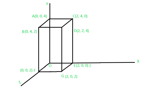
Fig.1

First, we perform translation transformation T1:

The Translation transformation matrix is shown as:

[Tex]\hspace{4.37cm}\mathbf{T_1=\left[\begin{matrix}1&0&0&0\\0&1&0&0\\0&0&1&0\\D_x&D_y&D_z&1\end{matrix}\right]}\\ \mathbf{Where \hspace{0.2cm}D_x=2,D_y=3\hspace{0.2cm} and\hspace{0.2cm} D_z=3\hspace{0.2cm} are\hspace{0.2cm}translation\hspace{0.2cm} distances.} [/Tex]

Now apply this translation transformation matrix condition over the coordinates:

For coordinate O[0 0 0], the newly translated coordinate would be O₁:

For coordinate A[0 0 4], the newly translated coordinate would be A₁:

For coordinate B[0 4 2], the newly translated coordinate would be B₁:

For coordinate C[2 4 0], the newly translated coordinate would be C₁:

For coordinate D[2 2 4], the newly translated coordinate would be D₁:

For coordinate E[2 0 0], the newly translated coordinate would be E₁:

For coordinate F[0 0 2], the newly translated coordinate would be F₁:

For coordinate G[2  0  2], the newly translated coordinate would be G₁:

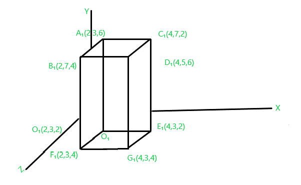
Fig.2

Secondly, we are said to perform Scaling transformation T₂:

The Scaling transformation matrix is shown as:

Now apply this Scaling transformation matrix condition over the coordinates:

For coordinate O₁[2 3 2], the newly Scaled coordinate would be O₂:

For coordinate A₁[2 3 6], the newly Scaled coordinate would be A₂:

For coordinate B₁[2 7 4], the newly Scaled coordinate would be B₂:

For coordinate C₁[4 7 2], the newly Scaled coordinate would be C₂:

For coordinate D₁[4 5 6], the newly Scaled coordinate would be D₂:

For coordinate E₁[4 3 2], the newly Scaled coordinate would be E₂:

For coordinate F₁[2 3 4], the newly Scaled coordinate would be F₂:

For coordinate G₁[4 3 4], the newly Scaled coordinate would be G₂:

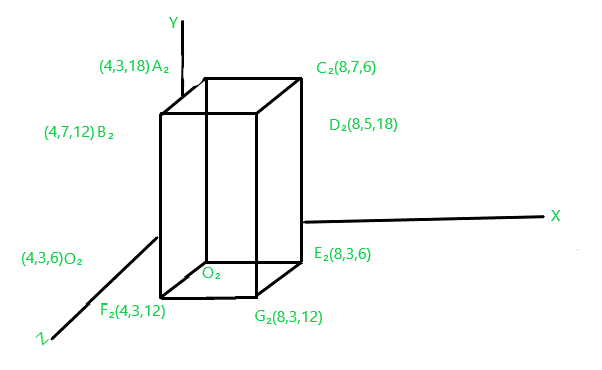
Fig.3

Lastly, we perform Shearing transformation T₃ in x-direction:

The Shearing transformation matrix for x-direction is shown as:

Now, apply this Shearing transformation matrix condition over the coordinates:

For coordinate O₂[4 3 6], the newly Scaled coordinate would be O₃:

For coordinate A₂[4  3 18], the newly Scaled coordinate would be A₃:

For coordinate B₂[4  7 12], the newly Scaled coordinate would be B₃:

For coordinate C₂[8  7  6], the newly Scaled coordinate would be C₃:

For coordinate D₂[8   5  18], the newly Scaled coordinate would be D₃:

For coordinate E₂[8  7  6], the newly Scaled coordinate would be E₃:

For coordinate F₂[4  3  12], the newly Scaled coordinate would be F₃:

For coordinate G₂[8  3 12], the newly Scaled coordinate would be G₃:

Finally, we get our resized slanted object in the x-direction after performing transformations T₁, T₂ and T₃.

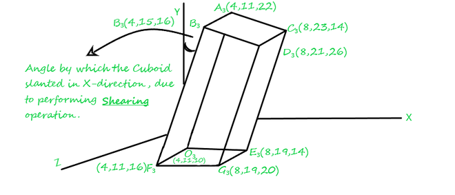
Fig.4

Solution through Composite Transformation

The final result, that we got above for the cuboid “OABCDEF” through applying transformation T₁, T₂, and T₃  one after one in sequential order the same equivalent result could also be got by using the concept of Composite Transformation. To perform composite transformation first we need to calculate the Resultant Transformation matrix(R) by combining all the distinguished transformation matrix representations together.

The resultant transformation matrix would be calculated as follows: 

The resultant transformation will be calculated by multiplying the Translation transformation matrix with the Scaling transformation matrix and the resultant(R₂) multiplication of both will then be multiplied with the last given, Shearing transformation matrix.

Now, multiply R2 with the Shearing transformation matrix to get resultant R:

\

Now, apply this resultant transformation matrix condition over the coordinates:

For coordinate O[0 0 0], the new Scaled coordinate would be O₃:

For coordinate A[0 0 4], the newly Scaled coordinate would be A₃:

For coordinate B[0 4 2], the newly Scaled coordinate would be B₃:

For coordinate C[2 4 0], the newly Scaled coordinate would be C₃:

For coordinate D[2  2  4], the newly Scaled coordinate would be D₃:

For coordinate E[2  0  0], the newly Scaled coordinate would be E₃:

For coordinate F[0  0  2], the newly Scaled coordinate would be F₃:

For coordinate G[2  0  2], the newly Scaled coordinate would be G₃:

Here, we get our final result in a single shot:

Fig.5