Computational Graph in PyTorch

PyTorch is a popular open-source machine learning library for developing deep learning models. It provides a wide range of functions for building complex neural networks. PyTorch defines a computational graph as a Directed Acyclic Graph (DAG) where nodes represent operations (e.g., addition, multiplication, etc.) and edges represent the flow of data between the operations. When defining a PyTorch model, the computational graph is created by defining the forward function of the model. This function takes inputs and applies a sequence of operations to produce the outputs. During the forward pass, PyTorch creates the computational graph by keeping track of the operations and their inputs and outputs.

A model’s calculation is represented by a graph, a type of data structure. A graph is represented in PyTorch by a directed acyclic graph (DAG), where each node denotes a calculation and each edge denotes the data flow between computations. In the backpropagation step, the graph is used to compute gradients and monitor the dependencies between computations.

A computational graph is a graphical representation of a mathematical function or algorithm, where the nodes of the graph represent mathematical operations, and the edges represent the input/output relationships between the operations. In other words, it is a way to visualize the flow of data through a system of mathematical operations.

Computational graphs are widely used in deep learning, where they serve as the backbone of neural networks. In a neural network, each node in the computational graph represents a neuron, and the edges represent the connections between neurons.

Implementations

Install the necessary libraries

sudo apt install graphviz   # [Ubuntu]
winget install graphviz     # [Windows]
sudo port install graphviz  # [Mac]

pip install torchviz

Step 1: Import  the necessary libraries

Python3

import torch
import torch.nn as nn
import torch.optim as optim
import torchvision.datasets as datasets
import torchvision.transforms as transforms
from torch.utils.data import DataLoader
from PIL import Image

from torchviz import make_dot

Step 2: Build the neural network model

Python3

# Define a neural network architecture
class Net(nn.Module):
    def __init__(self):
        super(Net, self).__init__()
        self.conv1 = nn.Conv2d(3, 16, 3)
        self.pool = nn.MaxPool2d(3, 2)
        self.fc1 = nn.Linear(238, 120)
        self.fc2 = nn.Linear(120,1)
        self.fc3 = nn.Sigmoid()

    def forward(self, x):
        x = self.pool(torch.relu(self.conv1(x)))
        x = x.view(-1, 238)
        x = torch.relu(self.fc1(x))
        x = torch.relu(self.fc2(x))
        x = torch.relu(self.fc3(x))
        return x

# Move the model to the GPU
device = torch.device("cuda:0" if torch.cuda.is_available() else "cpu")
net = Net().to(device)

Step 3: Load the image dataset 

Python3

# Load the image
img = Image.open("Ganesh.jpg")

# Transformation
transform = transforms.Compose([
    transforms.Resize((720, 480)),  # Resize the image to 720x480
    transforms.ToTensor(),
    transforms.Normalize((0.5, 0.5, 0.5), (0.5, 0.5, 0.5))
])

img = transform(img)
# Reshape the 4d tensor
img = img.view(1, 3, 720, 480)

# Move to GPU
img = img.to(device)
img.shape

Output:

torch.Size([1, 3, 720, 480])

Step 4: Process the first convolutional layer

Python3

# first convolutional layer
conv1 = net.conv1
print('Convolution Layer :',conv1)

# APPLY THE FIRST Convolutional layer to the image
y1 = conv1(img)
print('Output Shape :',y1.shape)

# Computational Graph
make_dot(y1, params=dict(net.named_parameters()))

Output:

Convolution Layer : Conv2d(3, 16, kernel_size=(3, 3), stride=(1, 1))
Output Shape : torch.Size([1, 16, 718, 478])

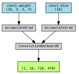
Computational Graph

Step 5: Process the Second Pooling layer

Python3

# Pooling layer
pool = net.pool
print('pooling Layer :',pool)

# APPLY THE Pooling layer to the
# output of FIRST Convolutional layer
y2 = pool(y1)
print('Output Shape :',y2.shape)

# Computational Graph
make_dot(y2, params=dict(net.named_parameters()))

Output:

pooling Layer : MaxPool2d(kernel_size=3, stride=2, padding=0, dilation=1, ceil_mode=False)
Output Shape : torch.Size([1, 16, 358, 238])

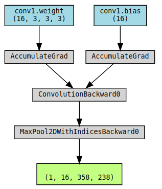
Computational Graph

Step 6: Process the first Linear layer

Python3

# first Linear layer
fc = net.fc1
print('First Linear Layer :',fc)

# APPLY THE Linear layer to the output y2
y3 = fc(y2)
print('Output Shape :',y3.shape)

# Computational Graph
make_dot(y3, params=dict(net.named_parameters()))

Output:

First Linear Layer : Linear(in_features=238, out_features=120, bias=True)
Output Shape : torch.Size([1, 16, 358, 120])

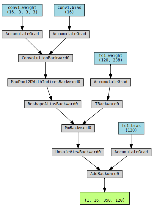
Computational Graph

Step 7: Process the second Linear layer

Python3

# Second Linear layer
fc_2 = net.fc2
print('Second Linear Layer :',fc_2)

# APPLY THE Second Linear layer to the output y3
y4 = fc_2(y3)
print('Output Shape :',y4.shape)

# Computational Graph
make_dot(y4, params=dict(fc_2.named_parameters()))

Output:

Second Linear Layer : Linear(in_features=120, out_features=1, bias=True)
Output Shape : torch.Size([1, 16, 358, 1])

Computational Graph

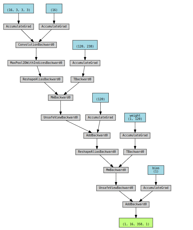
Step 8: Train the model and plot the final computational graph

Python3

# define labels
labels = torch.rand(1).to(device)

# forward propagation
prediction = net(img)

# define loss
loss = (prediction - labels).sum()

# backward pass
loss.backward()
# Optimizer
optimizer = optim.SGD(net.parameters(), lr=0.001, momentum=0.9)

# gradient descent
optimizer.step()

# Computational Graph
make_dot(prediction,
         params=dict(net.named_parameters()))

Output:

Computational Graph