Completely Randomized Design with R Programming

Experimental Designs are part of ANOVA in statistics. They are predefined algorithms that help us in analyzing the differences among group means in an experimental unit. Completely Randomized Design (CRD) is one part of the Anova types.

Completely Randomized Design:

The three basic principles of designing an experiment are replication, blocking, and randomization. In this type of design, blocking is not a part of the algorithm. The samples of the experiment are random with replications are assigned to different experimental units.  Let’s consider some experiments below and implement the experiment in R programming.

Experiment 1

Adding more baking powder to cakes increases the heights of the cake. Let’s see with CRD how the experiment will be analyzed. 

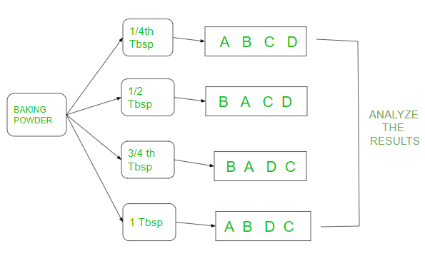
As shown in the above figure the baking powder is divided into 4 different tablespoons(tbsp) and four replicate cakes heights (respectively for A, B, C, D)  were made with each tbsp in random order. Then the results of tbsp are compared to see if actually the height is affected by baking powder. The replications are just permutations of the different cakes heights respectively for A, B, C, D. Let’s see the above example in R language. The heights of each cake are randomly noted for each tablespoon.

tbsp 0.25 0.5  0.75  1 
     1.4  7.8  7.6  1.6
  #(A,B,C,D)
     2.0  9.2  7.0  3.4
  #(A,B,D,C)
     2.3  6.8  7.3  3.0
  #(B,A,D,C)
     2.5  6.0  5.5  3.9  #(B,A,C,D)
  # the randomization is done directly by the program

The replications of the cakes are done with the below code:

R

treat <- rep(c("A", "B", "C", "D"), each = 4)
fac <- factor(rep(c(0.25, 0.5, 0.75, 1), each = 4))
treat

Output:

[1] A A A A B B B B C C C C D D D D
Levels: A B C D

Creating dataframe:

R

height <- c(1.4, 2.0, 2.3, 2.5,
              7.8, 9.2, 6.8, 6.0,
              7.6, 7.0, 7.3, 5.5,
              1.6, 3.4, 3.0, 3.9)

exp <- data.frame(treat, treatment = fac, response = height)
mod <- aov(response ~ treatment, data = exp)
summary(mod)

Output:

             Df Sum Sq Mean Sq F value Pr(>F)    
treatment    3  88.46  29.486   29.64 7.85e-06 ***
Residuals   12  11.94   0.995                     
---
Signif. codes:  0 ‘***’ 0.001 ‘**’ 0.01 ‘*’ 0.05 ‘.’ 0.1 ‘ ’ 1

Explanation:

For every experiment, the significance is either 0.05 or 0.01 which is given by the person taking the experiment. For this example, let’s consider the significance as 5% i.e 0.05. We should see the value of Pr(>F) which is 7.85e-06  ,i.e, < 0.05. Thus reject the hypothesis. If the value is > 0.05 then accept the hypothesis. For this example, as Pr < 0.05, reject the hypothesis. Let’s consider one more example:

Experiment 2

Adding rocks to water increases the height of water in the container. Let’s see this experiment in the figure as follows:

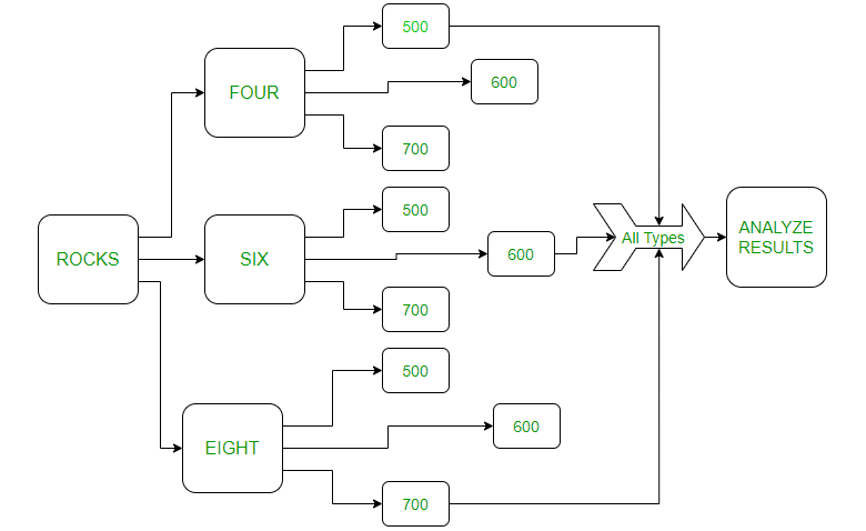
Consider that if adding four rocks to 500ml,600ml  and 700ml respectively increases the height of water correspondingly. For example: adding 6 rocks to 500 m water has  7 ms height increased.

rocks four six eight
 5    5.3  6.2 [500 600 700]
5.5    5   5.7 [600 500 700]
4.8   4.3  3.4 [700 600 500]

Lets code:

R

rocks<- rep(c("four", "six", "eight"), each = 3)
rocks
fac <- factor(rep(c(500, 600, 700), each = 3))
fac

Output:

[1] "four"  "four"  "four"  "six"   "six"   "six"   "eight" "eight" "eight"

[1] 500 500 500 600 600 600 700 700 700
Levels: 500 600 700

Creating dataframe:  

R

height <- c(5, 5.5, 4.8,
            5.3, 5, 4.3,
            4.8, 4.3, 3.4)
exp1 <- data.frame(rocks, treatment = fac,
                   response = height)
mod <- aov(response ~ treatment, data = exp1)
summary(mod)

Output:

Df Sum Sq Mean Sq F value Pr(>F)
treatment    2  1.416  0.7078   2.368  0.175
Residuals    6  1.793  0.2989 

Explanation:

Here 0.175>>0.05 thus hypothesis is accepted.