CNN | Introduction to Pooling Layer

The pooling operation involves sliding a two-dimensional filter over each channel of feature map and summarising the features lying within the region covered by the filter. 
For a feature map having dimensions n_h x n_w x n_c, the dimensions of output obtained after a pooling layer is 

(nh - f + 1) / s x (nw - f + 1)/s x nc

where, 

-> nh - height of feature map
-> nw - width of feature map
-> nc - number of channels in the feature map
-> f  - size of filter
-> s  - stride length

A common CNN model architecture is to have a number of convolution and pooling layers stacked one after the other. 

Why to use Pooling Layers?

• Pooling layers are used to reduce the dimensions of the feature maps. Thus, it reduces the number of parameters to learn and the amount of computation performed in the network.
• The pooling layer summarises the features present in a region of the feature map generated by a convolution layer. So, further operations are performed on summarised features instead of precisely positioned features generated by the convolution layer. This makes the model more robust to variations in the position of the features in the input image. 
  

Types of Pooling Layers:

Max Pooling

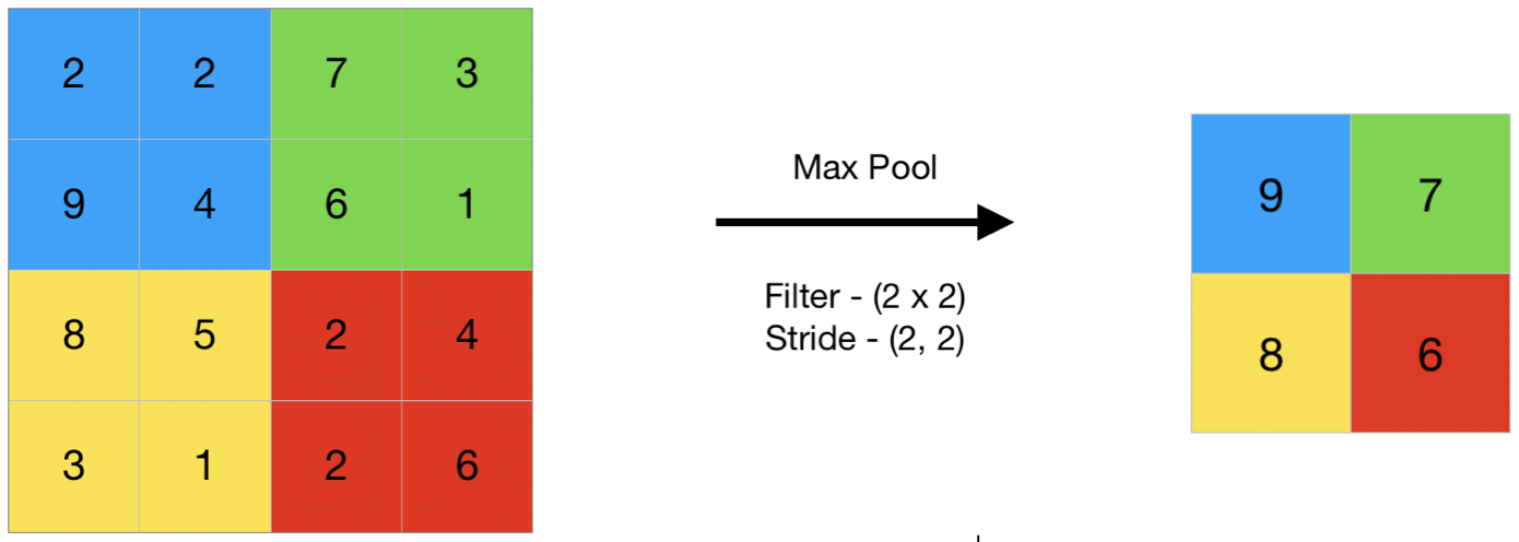
1. Max pooling is a pooling operation that selects the maximum element from the region of the feature map covered by the filter. Thus, the output after max-pooling layer would be a feature map containing the most prominent features of the previous feature map. 
   

1. This can be achieved using MaxPooling2D layer in keras as follows:
   Code #1 : Performing Max Pooling using keras

Python3

import numpy as np
from keras.models import Sequential
from keras.layers import MaxPooling2D

# define input image
image = np.array([[2, 2, 7, 3],
                  [9, 4, 6, 1],
                  [8, 5, 2, 4],
                  [3, 1, 2, 6]])
image = image.reshape(1, 4, 4, 1)

# define model containing just a single max pooling layer
model = Sequential(
    [MaxPooling2D(pool_size = 2, strides = 2)])

# generate pooled output
output = model.predict(image)

# print output image
output = np.squeeze(output)
print(output)

1. Output: 

[[9. 7.]
[8. 6.]]

Average Pooling

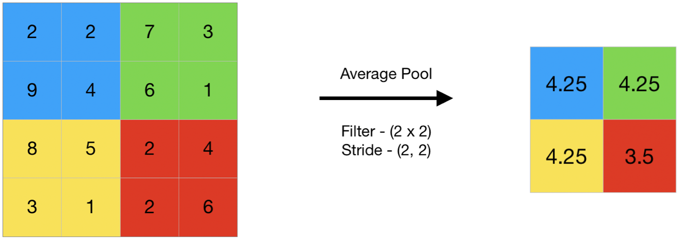
1. Average pooling computes the average of the elements present in the region of feature map covered by the filter. Thus, while max pooling gives the most prominent feature in a particular patch of the feature map, average pooling gives the average of features present in a patch. 
   

1. Code #2 : Performing Average Pooling using keras

Python3

import numpy as np
from keras.models import Sequential
from keras.layers import AveragePooling2D

# define input image
image = np.array([[2, 2, 7, 3],
                  [9, 4, 6, 1],
                  [8, 5, 2, 4],
                  [3, 1, 2, 6]])
image = image.reshape(1, 4, 4, 1)

# define model containing just a single average pooling layer
model = Sequential(
    [AveragePooling2D(pool_size = 2, strides = 2)])

# generate pooled output
output = model.predict(image)

# print output image
output = np.squeeze(output)
print(output)

1. Output: 

 
[[4.25 4.25]
[4.25 3.5 ]]

Global Pooling

1. Global pooling reduces each channel in the feature map to a single value. Thus, an n_h x n_w x n_c feature map is reduced to 1 x 1 x n_c feature map. This is equivalent to using a filter of dimensions n_h x n_w i.e. the dimensions of the feature map. 
   Further, it can be either global max pooling or global average pooling.
   Code #3 : Performing Global Pooling using keras

Python3

import numpy as np
from keras.models import Sequential
from keras.layers import GlobalMaxPooling2D
from keras.layers import GlobalAveragePooling2D

# define input image
image = np.array([[2, 2, 7, 3],
                  [9, 4, 6, 1],
                  [8, 5, 2, 4],
                  [3, 1, 2, 6]])
image = image.reshape(1, 4, 4, 1)

# define gm_model containing just a single global-max pooling layer
gm_model = Sequential(
    [GlobalMaxPooling2D()])

# define ga_model containing just a single global-average pooling layer
ga_model = Sequential(
    [GlobalAveragePooling2D()])

# generate pooled output
gm_output = gm_model.predict(image)
ga_output = ga_model.predict(image)

# print output image
gm_output = np.squeeze(gm_output)
ga_output = np.squeeze(ga_output)
print("gm_output: ", gm_output)
print("ga_output: ", ga_output)

1. Output: 

 
gm_output:  9.0
ga_output:  4.0625 

In convolutional neural networks (CNNs), the pooling layer is a common type of layer that is typically added after convolutional layers. The pooling layer is used to reduce the spatial dimensions (i.e., the width and height) of the feature maps, while preserving the depth (i.e., the number of channels).

1. The pooling layer works by dividing the input feature map into a set of non-overlapping regions, called pooling regions. Each pooling region is then transformed into a single output value, which represents the presence of a particular feature in that region. The most common types of pooling operations are max pooling and average pooling.
2. In max pooling, the output value for each pooling region is simply the maximum value of the input values within that region. This has the effect of preserving the most salient features in each pooling region, while discarding less relevant information. Max pooling is often used in CNNs for object recognition tasks, as it helps to identify the most distinctive features of an object, such as its edges and corners.
3. In average pooling, the output value for each pooling region is the average of the input values within that region. This has the effect of preserving more information than max pooling, but may also dilute the most salient features. Average pooling is often used in CNNs for tasks such as image segmentation and object detection, where a more fine-grained representation of the input is required.

Pooling layers are typically used in conjunction with convolutional layers in a CNN, with each pooling layer reducing the spatial dimensions of the feature maps, while the convolutional layers extract increasingly complex features from the input. The resulting feature maps are then passed to a fully connected layer, which performs the final classification or regression task.

Advantages of Pooling Layer:

1. Dimensionality reduction: The main advantage of pooling layers is that they help in reducing the spatial dimensions of the feature maps. This reduces the computational cost and also helps in avoiding overfitting by reducing the number of parameters in the model.
2. Translation invariance: Pooling layers are also useful in achieving translation invariance in the feature maps. This means that the position of an object in the image does not affect the classification result, as the same features are detected regardless of the position of the object.
3. Feature selection: Pooling layers can also help in selecting the most important features from the input, as max pooling selects the most salient features and average pooling preserves more information.

Disadvantages of Pooling Layer:

1. Information loss: One of the main disadvantages of pooling layers is that they discard some information from the input feature maps, which can be important for the final classification or regression task.
2. Over-smoothing: Pooling layers can also cause over-smoothing of the feature maps, which can result in the loss of some fine-grained details that are important for the final classification or regression task.
3. Hyperparameter tuning: Pooling layers also introduce hyperparameters such as the size of the pooling regions and the stride, which need to be tuned in order to achieve optimal performance. This can be time-consuming and requires some expertise in model building.