CIFAR-10 Image Classification in TensorFlow
Last Updated :
02 Nov, 2022
Prerequisites:
In this article, we are going to discuss how to classify images using TensorFlow. Image Classification is a method to classify the images into their respective category classes. CIFAR-10 Dataset as it suggests has 10 different categories of images in it. There is a total of 60000 images of 10 different classes naming Airplane, Automobile, Bird, Cat, Deer, Dog, Frog, Horse, Ship, Truck. All the images are of size 32×32. There are in total 50000 train images and 10000 test images.
To build an image classifier we make use of tensorflow‘ s keras API to build our model. In order to build a model, it is recommended to have GPU support, or you may use the Google colab notebooks as well.
Stepwise Implementation:
- The first step towards writing any code is to import all the required libraries and modules. This includes importing tensorflow and other modules like numpy. If the module is not present then you can download it using pip install tensorflow on the command prompt (for windows) or if you are using a jupyter notebook then simply type !pip install tensorflow in the cell and run it in order to download the module. Other modules can be imported similarly.
Python3
import tensorflow as tf
print(tf.__version__)
import numpy as np
import matplotlib.pyplot as plt
from tensorflow.keras.layers import Input, Conv2D, Dense, Flatten, Dropout
from tensorflow.keras.layers import GlobalMaxPooling2D, MaxPooling2D
from tensorflow.keras.layers import BatchNormalization
from tensorflow.keras.models import Model
|
Output:
2.4.1
The output of the above code should display the version of tensorflow you are using eg 2.4.1 or any other.
- Now we have the required module support so let’s load in our data. The dataset of CIFAR-10 is available on tensorflow keras API, and we can download it on our local machine using tensorflow.keras.datasets.cifar10 and then distribute it to train and test set using load_data() function.
Python3
cifar10 = tf.keras.datasets.cifar10
(x_train, y_train), (x_test, y_test) = cifar10.load_data()
print(x_train.shape, y_train.shape, x_test.shape, y_test.shape)
|
Output:
The output of the above code will display the shape of all four partitions and will look something like this

Here we can see we have 5000 training images and 1000 test images as specified above and all the images are of 32 by 32 size and have 3 color channels i.e. images are color images. As well as it is also visible that there is only a single label assigned with each image.
- Until now, we have our data with us. But still, we cannot be sent it directly to our neural network. We need to process the data in order to send it to the network. The first thing in the process is to reduce the pixel values. Currently, all the image pixels are in a range from 1-256, and we need to reduce those values to a value ranging between 0 and 1. This enables our model to easily track trends and efficient training. We can do this simply by dividing all pixel values by 255.0.
Another thing we want to do is to flatten(in simple words rearrange them in form of a row) the label values using the flatten() function.
Python3
x_train, x_test = x_train / 255.0, x_test / 255.0
y_train, y_test = y_train.flatten(), y_test.flatten()
|
- Now is a good time to see few images of our dataset. We can visualize it in a subplot grid form. Since the image size is just 32×32 so don’t expect much from the image. It would be a blurred one. We can do the visualization using the subplot() function from matplotlib and looping over the first 25 images from our training dataset portion.
Python3
fig, ax = plt.subplots(5, 5)
k = 0
for i in range(5):
for j in range(5):
ax[i][j].imshow(x_train[k], aspect='auto')
k += 1
plt.show()
|
Output:
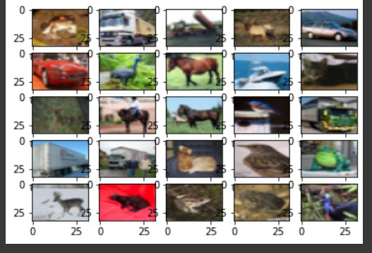
Though the images are not clear there are enough pixels for us to specify which object is there in those images.
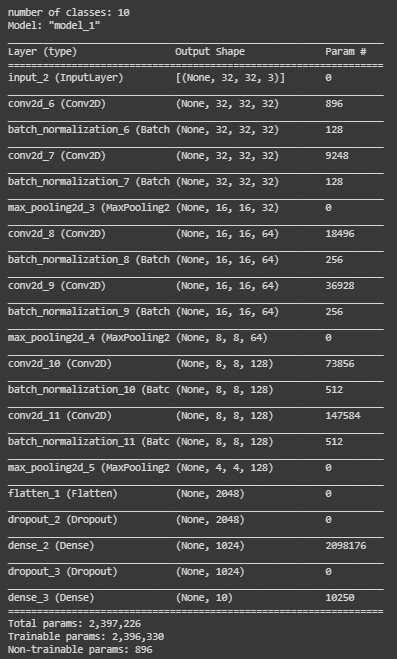
- After completing all the steps now is the time to built our model. We are going to use a Convolution Neural Network or CNN to train our model. It includes using a convolution layer in this which is Conv2d layer as well as pooling and normalization methods. Finally, we’ll pass it into a dense layer and the final dense layer which is our output layer. We are using ‘relu‘ activation function. The output layer uses a “softmax” function.
Python3
K = len(set(y_train))
print("number of classes:", K)
i = Input(shape=x_train[0].shape)
x = Conv2D(32, (3, 3), activation='relu', padding='same')(i)
x = BatchNormalization()(x)
x = Conv2D(32, (3, 3), activation='relu', padding='same')(x)
x = BatchNormalization()(x)
x = MaxPooling2D((2, 2))(x)
x = Conv2D(64, (3, 3), activation='relu', padding='same')(x)
x = BatchNormalization()(x)
x = Conv2D(64, (3, 3), activation='relu', padding='same')(x)
x = BatchNormalization()(x)
x = MaxPooling2D((2, 2))(x)
x = Conv2D(128, (3, 3), activation='relu', padding='same')(x)
x = BatchNormalization()(x)
x = Conv2D(128, (3, 3), activation='relu', padding='same')(x)
x = BatchNormalization()(x)
x = MaxPooling2D((2, 2))(x)
x = Flatten()(x)
x = Dropout(0.2)(x)
x = Dense(1024, activation='relu')(x)
x = Dropout(0.2)(x)
x = Dense(K, activation='softmax')(x)
model = Model(i, x)
model.summary()
|
Output:
Our model is now ready, it’s time to compile it. We are using model.compile() function to compile our model. For the parameters, we are using
- adam optimizer
- sparse_categorical_crossentropy as the loss function
- metrics=[‘accuracy’]
Python3
model.compile(optimizer='adam',
loss='sparse_categorical_crossentropy',
metrics=['accuracy'])
|
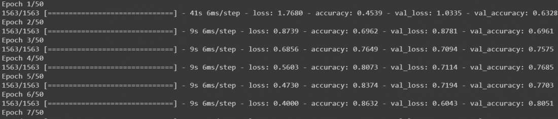
- Now let’s fit our model using model.fit() passing all our data to it. We are going to train our model till 50 epochs, it gives us a fair result though you can tweak it if you want.
Python3
r = model.fit(
x_train, y_train, validation_data=(x_test, y_test), epochs=50)
|
Output:
The model will start training, and it will look something like this
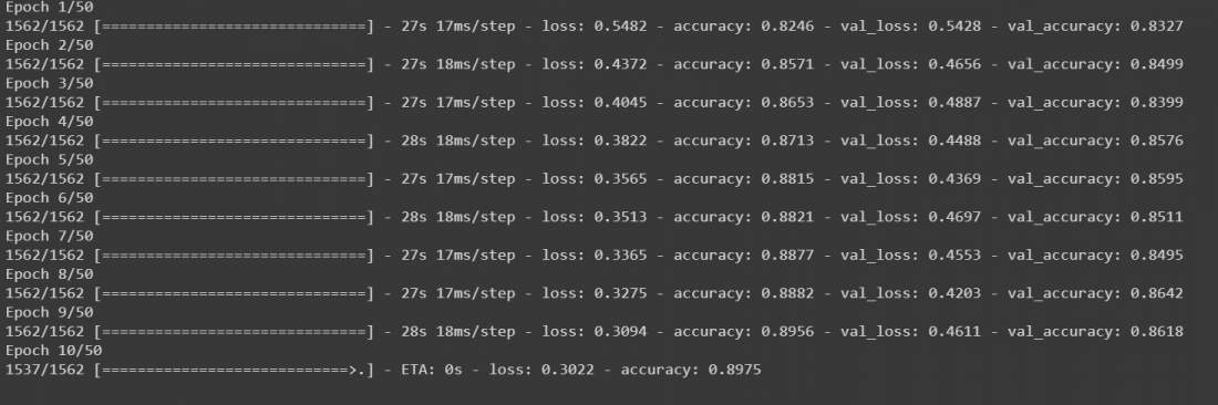
- After this, our model is trained. Though it will work fine but to make our model much more accurate we can add data augmentation on our data and then train it again. Calling model.fit() again on augmented data will continue training where it left off. We are going to fir our data on a batch size of 32 and we are going to shift the range of width and height by 0.1 and flip the images horizontally. Then call model.fit again for 50 epochs.
Python3
batch_size = 32
data_generator = tf.keras.preprocessing.image.ImageDataGenerator(
width_shift_range=0.1, height_shift_range=0.1, horizontal_flip=True)
train_generator = data_generator.flow(x_train, y_train, batch_size)
steps_per_epoch = x_train.shape[0] // batch_size
r = model.fit(train_generator, validation_data=(x_test, y_test),
steps_per_epoch=steps_per_epoch, epochs=50)
|
Output:
The model will start training for 50 epochs. Though it is running on GPU it will take at least 10 to 15 minutes.
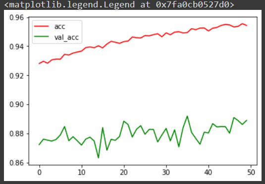
- Now we have trained our model, before making any predictions from it let’s visualize the accuracy per iteration for better analysis. Though there are other methods that include confusion matrix for better analysis of the model.
Python3
plt.plot(r.history['accuracy'], label='acc', color='red')
plt.plot(r.history['val_accuracy'], label='val_acc', color='green')
plt.legend()
|
Output:
Let’s make a prediction over an image from our model using model.predict() function. Before sending the image to our model we need to again reduce the pixel values between 0 and 1 and change its shape to (1,32,32,3) as our model expects the input to be in this form only. To make things easy let us take an image from the dataset itself. It is already in reduced pixels format still we have to reshape it (1,32,32,3) using reshape() function. Since we are using data from the dataset we can compare the predicted output and original output.
Python3
labels = .split()
image_number = 0
plt.imshow(x_test[image_number])
n = np.array(x_test[image_number])
p = n.reshape(1, 32, 32, 3)
predicted_label = labels[model.predict(p).argmax()]
original_label = labels[y_test[image_number]]
print("Original label is {} and predicted label is {}".format(
original_label, predicted_label))
|
Output:
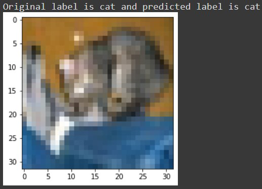
Now we have the output as Original label is cat and the predicted label is also cat.
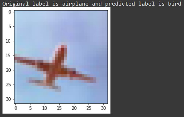
Let’s check it for some label which was misclassified by our model, e.g. for image number 5722 we receive something like this:
Finally, let’s save our model using model.save() function as an h5 file. If you are using Google colab you can download your model from the files section.
Python3
model.save('geeksforgeeks.h5')
|
Hence, in this way, one can classify images using Tensorflow.
Share your thoughts in the comments
Please Login to comment...