Change the position and the appearance of a graph legend in R

Legends are useful to add more information to the plots and enhance the user readability. It involves the creation of titles, indexes, placement of plot boxes in order to create a better understanding of the graphs plotted. The in-built R function legend() can be used to add a legend to the plot. Scatter, line and block plots are available for easy visualization of data in R. In this article, change the position and the appearance of a graph legend in R

Syntax: legend(x, y, legend)

Arguments :

• x and y : the x and y co-ordinates to be used to position the legend. It can also take string as an argument, like topright, bottomleft and so on..
• legend : vector giving info about each class plotted in the graph

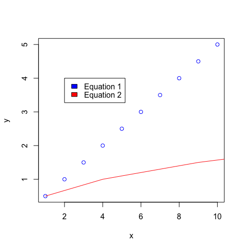
Example 1: Changing the Position of the legend 

Integer values can be assigned to both x and y coordinates and the legend box is aligned directly with these coordinates. It is necessary to provide both the coordinates in this case. 

Code:

R

# declaring the data to plot
# x coordinate is a vector of
# integers from 1 to 10
x <- 1 : 10
y = x^1/2
z =  x^2

# plotting x and y coordinate line
plot(x, y, col = "blue")

# adding another line on
# the coordinates involving y and z
lines(z, y ,col = "red")

# Adding a legend to the graph
#defining the lines
legend(2, 4, legend=c("Equation 1", "Equation 2"),
       fill = c("blue","red"))

Output:

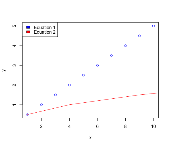
Example 2: Placement of legend with alignment justified.

The x coordinate may even contain a string with the position justified. The string is a combination of keywords, the plausible values of which are defined as bottomright, bottom, bottomleft, left, topleft, top, topright, right, center. This scenario eliminates the need of defining the value for y co-ordinate. 

Code:

R

# declaring the data to plot
# x coordinate is a vector of
# integers from 1 to 10

x <- 1 : 10
y = x^1/2
z =  x^2

# plotting x and y coordinate
# line
plot(x, y, col = "blue")

# adding another line on the
# coordinates involving y and z
lines(z, y , col = "red")

# Adding a legend to the graph
# defining the lines
legend(x = "topleft", legend=c(
  "Equation 1", "Equation 2"),
       fill = c("blue","red"))

Output

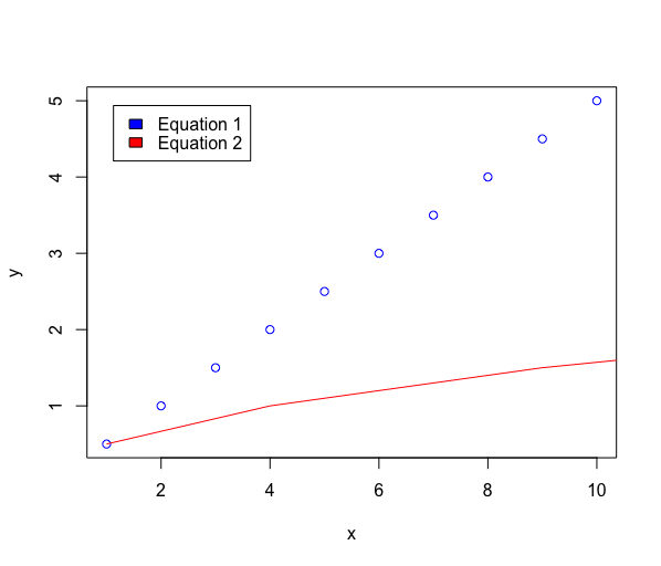
Example 3: Leaving margin along with alignment justification

In case, we specify the position argument in the form of keywords, the legend box appears connected to the corresponding axes. To resolve this, the inset argument can be defined within this method. This argument specifies the distance from the margin as a fraction of the plot region.

Code:

R

# declaring the data to plot
# x coordinate is a vector of
# integers from 1 to 10
x <- 1:10
y = x^1/2
z =  x^2

# plotting x and y coordinate line
plot(x, y, col = "blue")

# adding another line on the
# coordinates involving y and z
lines(z, y ,col = "red")

# Adding a legend to the graph
# defining the lines
legend(x="topleft", legend=c(
  "Equation 1", "Equation 2"),
       fill = c("blue","red"), inset = 0.05)

Output:

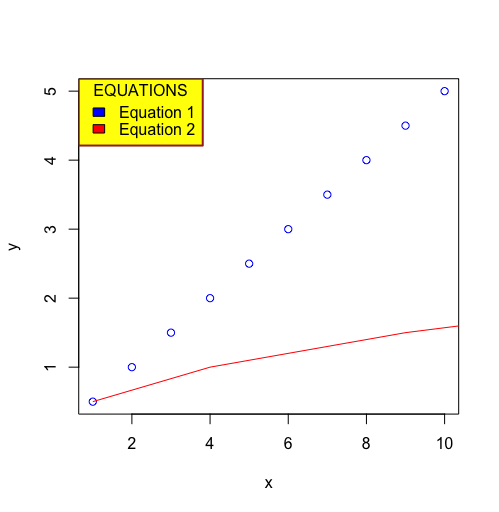
Example 4: Color appearance of the legend

The legend box in the graph can be customized to suit the requirements in order to convey more information and offer better visually. The following arguments can be used to customize the arguments.

• title: The title of the legend box that can be declared to understand what the index of the indicates
• bty (Default : o) : The type of box to enclose the legend . Different types of letters can be used, where the box shape is equivalent to the letter shape. For instance, “n” can be used for no box.
• bg: A background colour can be assigned to the legend box
• box.lwd : Indicator of the line width of the legend box
• box.lty : Indicator of the line type of the legend box
• box.col : Indicator of the line color of the legend box

Code:

R

# declaring the data to plot
# x coordinate is a vector of
# integers from 1 to 10
x <- 1:10
y = x^1/2
z = x^2

# plotting x and y coordinate line
plot(x, y, col = "blue")

# adding another line on the
# coordinates involving y and z
lines(z, y , col = "red")

# Adding a legend to the graph
# defining the lines
legend(x = "topleft", box.col = "brown",
       bg ="yellow", box.lwd = 2 , title="EQUATIONS",
       legend=c("Equation 1", "Equation 2"),
       fill = c("blue","red"))

Output: