Relative, Absolute and Mixed Cell Reference in Excel

Microsoft Excel, sometimes known as MS Excel, is a potent spreadsheet program. In Excel, each worksheet consists of a number of cells that are made up of rows and columns. Each cell has a unique reference, which enables users to quickly access and address the required cell (or cells) within the functions. In Excel, cell references are crucial, particularly when working with huge data sets in functions and formulas.

This article covers a quick overview of Excel Cell References. The various sorts of cell references that Excel offers and the detailed instructions for using each one are also covered in the article.

What is a Cell Reference?

An Excel cell reference, also known as a cell address, is a mechanism that defines a cell on a worksheet by combining a column letter and a row number. We can refer to any cell (in Excel formulas) in the worksheet by using the cell references.

For example:

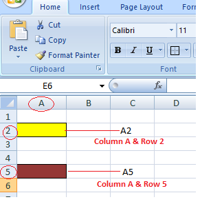
Here we refer to the cell in column A & row 2 by A2 & cell in column A & row 5 by A5. You can make use of such notations in any of the formulas or copy the value of one cell to another cell (by using = A2 or = A5).

Types of Cell Reference in Excel

Understanding various cell references primarily makes it easier for us to use Excel formulas and avoid unexpected formula errors. When copying and pasting Excel formulas, this is quite useful. Based on various use situations, Excel offers three main types of cell references, including:

• Relative Cell Reference
• Absolute Cell Reference
• Mixed Cell Reference

Relative Cell Reference 

In Excel, a relative cell reference is used by default. Excel uses a relative reference whenever we insert a cell reference or a range within a formula. The relative references, which commonly reflect the combination of column name and row number, are used normally with the associated cell references. There is no dollar ($) sign in the relative reference for the cell. 

How to Use Relative Cell References in Excel

Let’s see how to use the Relative Cell references through examples,

Example 1:

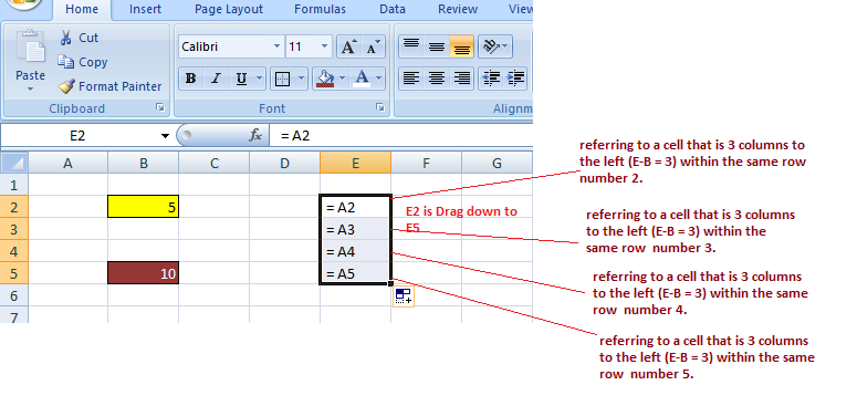
If you refer to cell B1 from cell E1, actually you would be referring to a cell that is 3 columns to the left (E-B = 3) within the same row number 1. 

When it is copied to other locations present in a worksheet, the relative reference for that location will be changed automatically. (because relative cell reference describes offset to another cell rather than a fixed address as In our example, offset is : 3 columns left in the same row).

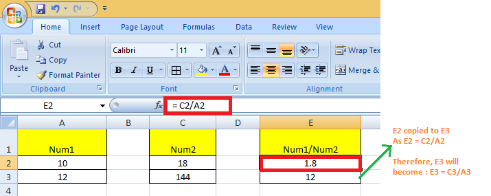
Example 2:

If you copy the formula = C2 / A2 from the cell “E2” to “E3”, the formula in E3 will automatically become =C3/A3.

When to Use Relative Cell References in Excel

When you need to develop a formula for a set of cells and the formula needs to make a reference to a relative cell reference, relative cell references come in handy.

When this occurs, you can create the formula in one cell and copy it before pasting it into every other cell.

Absolute Cell Reference 

When copying or using AutoFill, there are times when the cell reference must stay the same. A column and/or row reference is kept constant using dollar signs. So, to get an absolute reference from a relative, we can use the dollar sign ($) characters.

To refer to an actual fixed location on a worksheet whenever copying is done, we use absolute reference. The reference here is locked such that rows and columns do not shift when copied. 

How to Use Absolute Cell References in Excel

Below is an example depicting how to use Absolute Cell References in Excel.

Example :

When we fix both row & column – Say if we want to lock row 2 & column A, we will use $A$2 as:

G2 = C2/$A$2, when copied to G3, G3 becomes = C3/$A$2

 Note: C3 is 4 columns left to G3 in the same row.

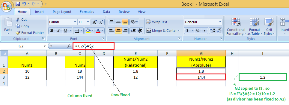
Here, original cell reference A2 is maintained whenever we copy G2 to any of the cells. So I3 = E3/$A$2 because E3 comes from the relative reference (4 columns left to the current one) & /$A$2 comes from the absolute reference.

Therefore, I3 = E3//$A$2 = 12/10 = 1.2

What Does the Dollar ($) Sign Do?

When the row and column numbers are preceded by the dollar symbol ($), it becomes absolute (i.e., stops the row and column number from changing when copied to other cells). Dollar ($) before the row fixes the row & before the column fixes the column.

When to Use Absolute Cell References in Excel

When you don’t want the cell reference to alter when you replicate formulas, absolute cell references come in handy. This can be the situation if you have to use a fixed value in the formula.

Mixed Cell Reference 

An absolute column and relative row, or an absolute row and relative column, is a mixed cell reference. You get an absolute column or absolute row when you individually put the $ before the column letter or before the row number. Example: $B8 is relative to row 8 but absolute for column B, and B$8 is absolute for row 1 but relative for column A.

Here, the Dollar ($) before the row number fixes/locks the row & before the column name fixes/locks the column.

Example

When we fix the only row: If we have G2 = C2/A$2 then :

We used $ before the row number, so we are locking the only row here. When G2 is copied to G3, G3 = C3/A$2 (not C3/A3) because the row has been fixed already.

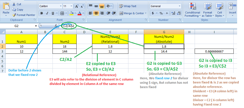
Here, whenever we copy G2 to any other cell, always the divisor will refer to a fixed row 2 (column vary according to the concept of relative reference)

So, when G2 is copied to I3, I3 = E3/C$2 because E3 comes from the relative reference (4 columns left to the current one) & C$2 comes from the absolute reference for row & relative reference for Column (6 Columns left to the current one)

Some Other Ways of Using Cell References With Examples

Now that we are familiar with the basics of using Cell References in Excel, let’s see some other ways of using cell references.

Relative and Absolute Cell References for Calculating Dates 

We can use relative and absolute cell references to calculate dates.

Example: To Calculate the Date of Delivery online from the given date of the order placed & no of days it will take to deliver :

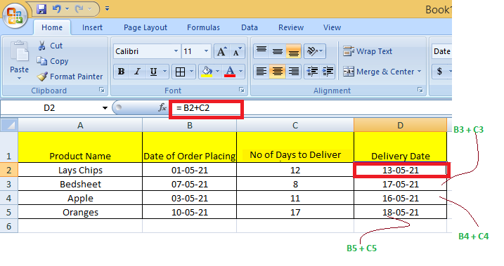
Here, We calculate the Date of Delivery by = Order Date + No of days to deliver. We used Relative cell reference so that individual product delivery dates can be calculated.

Absolute cell references for calculating dates :

Example: To Calculate the Date of Birth When the age is known is a number of days using Current date can be done by making use of absolute reference. 

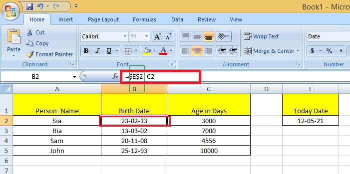
Here, We calculate DOB by = Current Date – Age in days. The Current date is contained in the cell E2 & in subtraction, we fixed that date to subtract from the days.

Whole Column Reference 

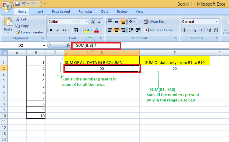
You will want to refer to all the cells inside a particular column when operating with an Excel worksheet with any number of rows. Simply type a column letter twice with a colon in between to refer to the entire column B, for example, B:B.

Example: You may want to find the sum of a column of data in certain cases. While you can do this with a regular cell range, such as =SUM(B1:B10), you will need to change the cell range if your spreadsheet grows in size.

Excel, on the other hand, has a cell range that does not require the row number and takes all the cells in the column in action. If you wanted to find the sum of all the values in column B, for example, you would type =SUM (B:B). You can add as much data as you want to your spreadsheet without having to change your cell ranges if you use this type of cell range.

Whole Row Reference 

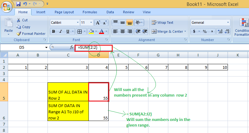
You will want to refer to all the cells inside a particular row when operating with an Excel worksheet with any number of columns. Simply type a row number twice with a colon in between to refer to the entire row, for example, 2:2.

Example: You may want to find the sum of a row of data in certain cases. While you can do this with a regular cell range, such as =SUM(A2 : J2), you will need to change the cell range if your spreadsheet grows in size.

Excel, on the other hand, has a cell range that does not require the column letter and takes all the cells in the row in action. If you wanted to find the sum of all the values in row 2, for example, you would type =SUM (2:2). You can add as much data as you want to your spreadsheet without having to change your cell ranges if you use this type of cell range.

Refer to an Entire Column, Excluding the First Few Rows 

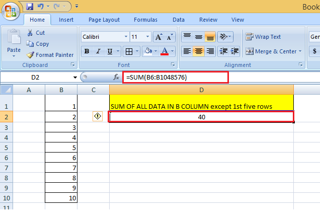
To refer to the entire column excluding the first few rows, you need to specify the range as we give in a normal fashion. We know that the Excel worksheets can have only 1,048,576 rows. (To check this, go to an empty cell & press: Ctrl + Down arrow Key)

So, we can do the sum of the entire column B except for the first 5 rows by = SUM(B6:B1048576).

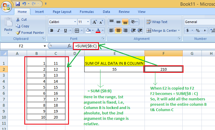
Using a Mixed Entire Column Reference in Excel 

You can also create a mixed entire-column reference, say for example $B:B. But, practically, it is difficult to find a situation where it would be used.

Example :

How to switch between Absolute, Relative, and Mixed References

The $ sign can be manually typed in an Excel formula to adjust a relative cell relation to absolute or mixed. You can also speed things up by pressing the F4 key. You must be in formula edit mode to use the F4 shortcut. The steps are :
Firstly, choose the cell that contains the formula. Then, by pressing the F2 key or double-clicking the cell, you can enter Edit mode. Select the cell reference in which you want to make changes. Then, switch between four-cell reference forms by pressing F4.

Example: When you select a cell having only relative reference (i.e., no $ sign), say = B2:

• The first time when you press F4, it becomes =$B$2
• The second time when you press F4, it becomes =B$2
• The third time when you press F4, it becomes=$B2
• The fourth time when you press F4, it becomes back to the relative reference=B2

B2 –Press F4–> =$B$2  –Press F4–> =B$2 –Press F4–> = =$B2  –Press F4–> =B2

So, using F4, you do not require to manually type the $ symbol.

Cell Reference to Other Worksheets

Cell reference in Excel are not limited to just the current worksheet. You can also reference cells from other worksheets within the same workbook. Let’s walk through an example to understand how to create these references.

Suppose we have two worksheets : “Sheet1” and “Sheet 2”. In “Sheet 2” we have value Student name that we want reference in “Sheet 1”.

Follow the below steps to create direct reference to “Sheet 2” from “Sheet 1”:

Step 1: Activate a cell in “Sheet 1” where you want to display the referenced value.

Step 2: Type an equal sign(=) in that cell to start a formula or reference.

Step 3: Switch to “Sheet 2” by clicking on its tab at the bottom of the Excel window.

Step 4: Locate the Specific cell that contains the desired value.

Step 5: Click on that cell to include it in the reference.

Step 6: Press Enter to complete the reference.

Once you press Enter, a reference is created in “Sheet 1” that points to the corresponding cell in “Sheet 2”. This means that any changes made to the referenced cell in “Sheet 2” will automatically reflect in the referenced value within “Sheet 1”.

Important Points to Remember

• One of the crucial components for Excel functions or formulas is the cell reference.
• Excel formulas that employ relative cell references automatically change the references to match the correct row and column.
• When copying formulas into non-relative cells, absolute cell references are advised. Excel keeps the absolute cell references constant.
• According to the specifications, a mixed reference only locks one of the references, either the row or the column. Not both are locked.

FAQs on Excel Cell References 

What is Cell Reference in Excel?

Cell Reference in Excel is a alphanumeric value that means it consists of combination of column letter and a row number that identifies a specific cell on a worksheet. It is used to refer to or manipulate data within that cell.

How we can create a cell reference in Excel?

To create a cell reference, you can simply type the column letter followed by the row number in a formula or function.

When we can use mixed cell reference in Excel?

Mixed cell references are useful when you want to fix either the column or the row while allowing the other part to adjust when copied.